Scott Sumner | Uneasy Money

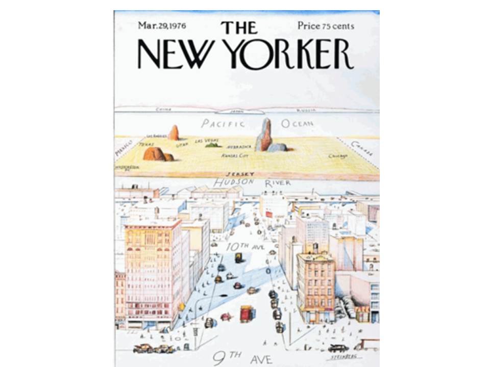
Posts Tagged 'Scott Sumner'

Can We All Export Our Way out of Depression?

Tyler Cowen has a post chastising Keynesians for scolding Germany for advising their Euro counterparts to adopt the virtuous German example of increasing their international competitiveness so that they can increase their exports, thereby increasing GDP and employment. The Keynesian response is that increasing exports is a zero-sum game, so that, far from being a recipe for recovery, the German advice is actually a recipe for continued stagnation.

Tyler doesn’t think much of the Keynesian response.

But that Keynesian counter is a mistake, perhaps brought on by the IS-LM model and its impoverished treatment of banking and credit.

Let’s say all nations could indeed increase their gross exports, although of course the sum of net exports could not go up. The first effect is that small- and medium-sized enterprises would be more profitable in the currently troubled economies. They would receive more credit and the broader monetary aggregates would go up in those countries, reflating their economies. (Price level integration is not so tight in these cases, furthermore much of the reflation could operate through q’s rather than p’s.) It sometimes feels like the IS-LM users have a mercantilist gold standard model, where the commodity base money can only be shuffled around in zero-sum fashion and not much more can happen in a positive direction.

The problem with Tyler’s rejoinder to the Keynesian response, which, I agree, provides an incomplete picture of what is going on, is that he assumes that which he wants to prove, thereby making his job just a bit too easy. That is, Tyler just assumes that “all nations could indeed increase their gross exports.” Obviously, if all nations increase their gross exports, they will very likely all increase their total output and employment. (It is, I suppose, theoretically possible that all the additional exports could be generated by shifting output from non-tradables to tradables, but that seems an extremely unlikely scenario.) The reaction of credit markets and monetary aggregates would be very much a second-order reaction. It’s the initial assumption– that all nations could increase gross exports simultaneously — that is doing all the heavy lifting.

Concerning Tyler’s characterization of the IS-LM model as a mercantilist gold-standard model, I agree that IS-LM has serious deficiencies, but that characterization strikes me as unfair. The simple IS-LM model is a closed economy model, with an exogenously determined price level. Such a model certainly has certain similarities to a mercantilist gold standard model, but that doesn’t mean that the two models are essentially the same. There are many ways of augmenting the IS-LM model to turn it into an open-economy model, in which case it would not necessarily resemble the a mercantilist gold-standard model.

Now I am guessing that Tyler would respond to my criticism by asking: “well, why wouldn’t all countries increase their gross exports is they all followed the German advice?”

My response to that question would be that the conclusion that everybody’s exports would increase if everybody became more efficient logically follows only in a comparative-statics framework. But, for purposes of this exercise, we are not starting from an equilibrium, and we have no assurance that, in a disequilibrium environment, the interaction of the overall macro disequilibrium with the posited increase of efficiency would produce, as the comparative-statics exercise would lead us to believe, a straightforward increase in everyone’s exports. Indeed, even the comparative-statics exercise is making an unsubstantiated assumption that the initial equilibrium is locally unique and stable.

Of course, this response might be dismissed as a mere theoretical possibility, though the likelihood that widespread adoption of export-increasing policies in the midst of an international depression, unaccompanied by monetary expansion, would lead to increased output does not seem all that high to me. So let’s think about what might happen if all countries simultaneously adopted export-increasing policies. The first point to consider is that not all countries are the same, and not all are in a position to increase their exports by as much or as quickly as others. Inevitably, some countries would increase their exports faster than others. As a result, it is also inevitable that some countries would lose export markets as other countries penetrated export markets before they did. In addition, some countries would experience declines in domestic output as domestic-import competing industries were forced by import competition to curtail output. In the absence of demand-increasing monetary policies, output and employment in some countries would very likely fall. This is the kernel of truth in the conventional IS-LM analysis that Tyler tries to dismiss. The IS-LM framework abstracts from the output-increasing tendency of export-led growth, but the comparative-statics approach abstracts from aggregate-demand effects that could easily overwhelm the comparative-statics effect.

Now, to be fair, I must acknowledge that Tyler reaches a pretty balanced conclusion:

This interpretation of the meaning of zero-sum net exports is one of the most common economic mistakes you will hear from serious economists in the blogosphere, and yet it is often presented dogmatically or dismissively in a single sentence, without much consideration of more complex or more realistic scenarios.

That is a reasonable conclusion, but I think it would be just as dogmatic, if not more so, to rely on the comparative-statics analysis that Tyler goes through in the first part of his post without consideration of more complex or more realistic scenarios.

Let me also offer a comment on Scott Sumner’s take on Tyler’s post. Scott tries to translate Tyler’s analysis into macroeconomic terms to support Tyler’s comparative-statics analysis. Scott considers three methods by which exports might be increased: 1) supply-side reforms, 2) monetary stimulus aimed at currency depreciation, and 3) increased government saving (fiscal austerity). The first two, Scott believes, lead to increased output and employment, and that the third is a wash. I agree with Scott about monetary stimulus aimed at currency depreciation, but I disagree (at least in part) about the other two.

Supply-side reforms [to increase exports] boost output under either an inflation target, or a dual mandate. If you want to use the Keynesian model, these reforms boost the Wicksellian equilibrium interest rate, which makes NGDP grow faster, even at the zero bound.

Scott makes a fair point, but I don’t think it is necessarily true for all inflation targets. Here is how I would put it. Because supply-side reforms to increase exports could cause aggregate demand in some countries to fall, and we have very little ability to predict by how much aggregate demand could go down in some countries adversely affected by increased competition from exports by other countries, it is at least possible that worldwide aggregate demand would fall if such policies were generally adopted. You can’t tell how the Wicksellian natural rate would be affected until you’ve accounted for all the indirect feedback effects on aggregate demand. If the Wicksellian natural rate fell, an inflation target, even if met, might not prevent a slowdown in NGDP growth, and a net reduction in output and employment. To prevent a slowdown in NGDP growth would require increasing the inflation target. Of course, under a real dual mandate (as opposed to the sham dual mandate now in place at the Fed) or an NGDP target, monetary policy would have to be loosened sufficiently to prevent output and employment from falling.

As far as government saving (fiscal austerity), I’d say it’s a net wash, for monetary offset reasons.

I am not sure what Scott means about monetary offset in this context. As I have argued in several earlier posts (here, here, here and here), attempting to increase employment via currency depreciation and increased saving involves tightening monetary policy, not loosening it. So I don’t see how fiscal policy can be used to depreciate a currency at the same time that monetary policy is being loosened. At any rate, if monetary policy is being used to depreciate the currency, then I see no difference between options 2) and 3).

But my general comment is that, like Tyler, Scott seems to be exaggerating the difference between his bottom line and the one that comes out of the IS-LM model, though I am certainly not saying that IS-LM is last word on the subject.

Responding to Scott Sumner

Published September 14, 2014 coordination failure , Nick Rowe , Scott Sumner 12 Comments
Tags: Nick Rowe, Scott Sumner

Scott Sumner cites this passage from my previous post about coordination failures.

I can envision a pure barter economy with incorrect price expectations in which individual plans are in a state of discoordination. Or consider a Fisherian debt-deflation economy in which debts are denominated in terms of gold and gold is appreciating. Debtors restrict consumption not because they are trying to accumulate more cash but because their debt burden is so great, any income they earn is being transferred to their creditors. In a monetary economy suffering from debt deflation, one would certainly want to use monetary policy to alleviate the debt burden, but using monetary policy to alleviate the debt burden is different from using monetary policy to eliminate an excess demand for money. Where is the excess demand for money?

Evidently, Scott doesn’t quite find my argument that coordination failures are possible, even without an excess demand for money, persuasive. So he puts the following question to me.

Why is it different from alleviating an excess demand for money?

I suppose that my response is this is: I am not sure what the question means. Does Scott mean to say that he does not accept that in my examples there really is no excess demand for money? Or does he mean that the effects of the coordination failure are no different from what they would be if there were an excess demand for money, any deflationary problem being treatable by increasing the quantity of money, thereby creating an excess supply of money. If Scott’s question is the latter, then he might be saying that the two cases are observationally equivalent, so that my distinction between a coordination failure with an excess demand for money and a coordination failure without an excess demand for money is really not a difference worth making a fuss about. The first question raises an analytical issue; the second a pragmatic issue.

Scott continues:

As far as I know the demand for money is usually defined as either M/P or the Cambridge K. In either case, a debt crisis might raise the demand for money, and cause a recession if the supply of money is fixed. Or the Fed could adjust the supply of money to offset the change in the demand for money, and this would prevent any change in AD, P, and NGDP.

I don’t know what Scott means when he says that the demand for money is usually defined as M/P. M/P is a number of units of currency. The demand for money is some functional relationship between desired holdings of money and a list of variables that influence those desired holdings. To say that the demand for money is defined as M/P is to assert an identity between the amount of money demanded and the amount in existence which rules out an excess demand for money by definition, so now I am really confused. The Cambridge k expresses the demand for money in terms of a desired relationship between the amount of money held and nominal income. But again, I can’t tell whether Scott is thinking of k as a functional relationship that depends on a list of variables or as a definition in which case the existence of an excess demand for money is ruled out by definition. So I am still confused.

I agree that a debt crisis could raise the demand for money, but in my example, it is entirely plausible that, on balance, the demand for money to hold went down because debtors would have to use all their resources to pay the interest owed on their debts.

I don’t disagree that the Fed could engage in a monetary policy that would alleviate the debt burden, but the problem they would be addressing would not be an excess demand for money; the problem being addressed would be the debt burden. but under a gold clause inflation wouldn’t help because creditors would be protected from inflation by the requirement that they be repaid in terms of a constant gold value.

Scott concludes:

Perhaps David sees the debt crisis working through supply-side channels—causing a recession despite no change in NGDP. That’s possible, but it’s not at all clear to me that this is what David has in mind.

The case I had in mind may or may not be associated with a change in NGDP, but any change in NGDP was not induced by an excess demand for money; it was induced by an increase in the value of gold when debts were denominated, as they were under the gold clause, in terms of gold.

I hope that this helps.

PS I see that Nick Rowe has a new post responding to my previous post. I have not yet read it. But it is near the top of my required reading list, so I hope to have a response for him in the next day or two.

The Trouble with IS-LM (and its Successors)

Published August 22, 2014 Bertil Ohlin , David Laidler , expectations , IS-LM , Keynes , macroeconomics , Roger Backhouse , Stockholm School 14 Comments
Tags: IS-LM, Keynes, Scott Sumner, Stockholm School

Lately, I have been reading a paper by Roger Backhouse and David Laidler, “What Was Lost with IS-LM” (an earlier version is available here) which was part of a very interesting symposium of 11 papers on the IS-LM model published as a supplement to the 2004 volume of History of Political Economy. The main thesis of the paper is that the IS-LM model, like the General Theory of which it is a partial and imperfect distillation, aborted a number of promising developments in the rapidly developing, but still nascent, field of macroeconomics in the 1920 and 1930s, developments that just might, had they not been elbowed aside by the IS-LM model, have evolved into a more useful and relevant theory of macroeconomic fluctuations and policy than we now possess. Even though I have occasionally sparred with Scott Sumner about IS-LM – with me pushing back a bit at Scott’s attacks on IS-LM — I have a lot of sympathy for the Backhouse-Laidler thesis.

The Backhouse-Laidler paper is too long to summarize, but I will just note that there are four types of loss that they attribute to IS-LM, which are all, more or less, derivative of the static equilibrium character of Keynes’s analytic method in both the General Theory and the IS-LM construction.

1 The loss of dynamic analysis. IS-LM is a single-period model.

2 The loss of intertemporal choice and expectations. Intertemporal choice and expectations are excluded a priori in a single-period model.

3 The loss of policy regimes. In a single-period model, policy is a one-time affair. The problem of setting up a regime that leads to optimal results over time doesn’t arise.

4 The loss of intertemporal coordination failures. Another concept that is irrelevant in a one-period model.

There was one particular passage that I found especially impressive. Commenting on the lack of any systematic dynamic analysis in the GT, Backhouse and Laidler observe,

[A]lthough [Keynes] made many remarks that could be (and in some cases were later) turned into dynamic models, the emphasis of the General Theory was nevertheless on unemployment as an equilibrium phenomenon.

Dynamic accounts of how money wages might affect employment were only a little more integrated into Keynes’s formal analysis than they were later into IS-LM. Far more significant for the development in Keynes’s thought is how Keynes himself systematically neglected dynamic factors that had been discussed in previous explanations of unemployment. This was a feature of the General Theory remarked on by Bertil Ohlin (1937, 235-36):

Keynes’s theoretical system . . . is equally “old-fashioned” in the second respect which characterizes recent economic theory – namely, the attempt to break away from an explanation of economic events by means of orthodox equilibrium constructions. No other analysis of trade fluctuations in recent years – with the possible exception of the Mises-Hayek school – follows such conservative lines in this respect. In fact, Keynes is much more of an “equilibrium theorist” than such economists as Cassel and, I think, Marshall.

Backhouse and Laidler go on to cite the Stockholm School (of which Ohlin was a leading figure) as an example of explicitly dynamic analysis.

As Bjorn Hansson (1982) has shown, this group developed an explicit method, using the idea of a succession of “unit periods,” in which each period began with agents having plans based on newly formed expectations about the outcome of executing them, and ended with the economy in some new situation that was the outcome of executing them, and ended with the economy in some new situation that was the outcome of market processes set in motion by the incompatibility of those plans, and in which expectations had been reformulated, too, in the light of experience. They applied this method to the construction of a wide variety of what they called “model sequences,” many of which involved downward spirals in economic activity at whose very heart lay rising unemployment. This is not the place to discuss the vexed question of the extent to which some of this work anticipated the Keynesian multiplier process, but it should be noted that, in IS-LM, it is the limit to which such processes move, rather than the time path they follow to get there, that is emphasized.

The Stockholm method seems to me exactly the right way to explain business-cycle downturns. In normal times, there is a rough – certainly not perfect, but good enough — correspondence of expectations among agents. That correspondence of expectations implies that the individual plans contingent on those expectations will be more or less compatible with one another. Surprises happen; here and there people are disappointed and regret past decisions, but, on the whole, they are able to adjust as needed to muddle through. There is usually enough flexibility in a system to allow most people to adjust their plans in response to unforeseen circumstances, so that the disappointment of some expectations doesn’t become contagious, causing a systemic crisis.

But when there is some sort of major shock – and it can only be a shock if it is unforeseen – the system may not be able to adjust. Instead, the disappointment of expectations becomes contagious. If my customers aren’t able to sell their products, I may not be able to sell mine. Expectations are like networks. If there is a breakdown at some point in the network, the whole network may collapse or malfunction. Because expectations and plans fit together in interlocking networks, it is possible that even a disturbance at one point in the network can cascade over an increasingly wide group of agents, leading to something like a system-wide breakdown, a financial crisis or a depression.

But the “problem” with the Stockholm method was that it was open-ended. It could offer only “a wide variety” of “model sequences,” without specifying a determinate solution. It was just this gap in the Stockholm approach that Keynes was able to fill. He provided a determinate equilibrium, “the limit to which the Stockholm model sequences would move, rather than the time path they follow to get there.” A messy, but insightful, approach to explaining the phenomenon of downward spirals in economic activity coupled with rising unemployment was cast aside in favor of the neater, simpler approach of Keynes. No wonder Ohlin sounds annoyed in his comment, quoted by Backhouse and Laidler, about Keynes. Tractability trumped insight.

Unfortunately, that is still the case today. Open-ended models of the sort that the Stockholm School tried to develop still cannot compete with the RBC and DSGE models that have displaced IS-LM and now dominate modern macroeconomics. The basic idea that modern economies form networks, and that networks have properties that are not reducible to just the nodes forming them has yet to penetrate the trained intuition of modern macroeconomists. Otherwise, how would it have been possible to imagine that a macroeconomic model could consist of a single representative agent? And just because modern macroeconomists have expanded their models to include more than a single representative agent doesn’t mean that the intellectual gap evidenced by the introduction of representative-agent models into macroeconomic discourse has been closed.

The Backing Theory of Money v. the Quantity Theory of Money

Published June 9, 2014 backing theory of money , Ben Klein , quantity theory of money , Scott Sumner 36 Comments
Tags: Ben Klein, Mike Sproul, Nick Rowe, Scott Sumner

Mike Sproul and Scott Sumner were arguing last week about how to account for the value of fiat money and the rate of inflation. As I observed in a recent post, I am doubtful that monetary theory, in its current state, can handle those issues adequately, so I am glad to see that others are trying to think the problems through even if the result is only to make clear how much we don’t know. Both Mike and Scott are very smart guys, and I find some validity in the arguments of both even if I am not really satisfied with the arguments of either.

Mike got things rolling with a guest post on JP Koning’s blog in which he lodged two complaints against Scott:

First, “Scott thinks that the liabilities of governments and central banks are not really liabilities.”

I see two problems with Mike’s first complaint. First, Mike is not explicit about which liabilities he is referring to. However, from the context of his discussion, it seems clear that he is talking about those liabilities that we normally call currency, or in the case of the Federal Reserve, Federal Reserve Notes. Second, and more important, it is not clear what definition of “liability” Mike is using. In a technical sense, as Mike observes, Federal Reserve Notes are classified by the Fed itself as liabilities. But what does it mean for a Federal Reserve Note to be a liability of the Fed? A liability implies that an obligation has been undertaken by someone to be discharged under certain defined conditions. What is the obligation undertaken by the Fed upon issuing a Federal Reserve Note. Under the gold standard, the Fed was legally obligated to redeem its Notes for gold at a fixed predetermined conversion rate. After the gold standard was suspended, that obligation was nullified. What obligation did the Fed accept in place of the redemption obligation? Here’s Mike’s answer:

But there are at least three other ways that FRN’s can still be redeemed: (i) for the Fed’s bonds, (ii) for loans made by the Fed, (iii) for taxes owed to the federal government. The Fed closed one channel of redemption (the gold channel), while the other redemption channels (loan, tax, and bond) were left open.

Those are funny obligations inasmuch as there are no circumstances under which they require the Fed to take any action. The purchase of a Fed (Treasury?) bond at the going market price imposes no obligation on the Fed to do anything except what it is already doing anyway. For there to be an obligation resulting from the issue by the Fed of a note, it would have been necessary for the terms of the transaction following upon the original issue to have been stipulated in advance. But the terms on which the Fed engages in transactions with the public are determined by market forces not by contractual obligation. The same point applies to loans made by the Fed. When the Fed makes a loan, it emits FRNs. The willingness of the Fed to accept FRNs previously emitted in the course of making loans as repayment of those loans doesn’t strike me as an obligation associated with its issue of FRNs. Finally, the fact that the federal government accepts (or requires) payment of tax obligations in FRNs is a decision of the Federal government to which the Fed as a matter of strict legality is not a party. So it seems to me that the technical status of an FRN as a liability of the Fed is a semantic or accounting oddity rather than a substantive property of a FRN.

Having said that, I think that Mike actually does make a substantive point about FRNs, which is that FRNs are not necessarily hot potatoes in the strict quantity-theory sense. There are available channels through which the public can remit its unwanted FRNs back to the Fed. The economic question is whether those means of sending unwanted FRNs back to the Fed are as effective in pinning down the price level as an enforceable legal obligation undertaken by the Fed to redeem FRNs at a predetermined exchange rate in terms of gold. Mike suggests that the alternative mechanisms by which the public can dispose of unwanted FRNs are as effective as gold convertibility in pinning down the price level. I think that assertion is implausible, and it remains to be proved, though I am willing to keep an open mind on the subject.

Now let’s consider Mike’s second complaint: “Scott thinks that if the central bank issues more money, then the money will lose value even if the money is fully backed.”

My first reaction is to ask what it means for money to be “fully backed?” Since it is not clear in what sense the inconvertible note issue of a central bank represents a liability of the issuing bank, it is also not exactly clear why any backing is necessary, or what backing means, though I will try to suggest in a moment a reason why the assets of the central bank actually do matter. But again the point is that, when a liability does not impose a well-defined legal obligation on the central bank to redeem that liability at a predetermined rate in terms of an asset whose supply the central bank does not itself control, the notion of “backing” is as vague as the notion of a “liability.” The difference between a liability that imposes no effective constraint on a central bank and one that does impose an effective constraint on a central bank is the difference between what Nick Rowe calls an alpha bank, which does not make its notes convertible into another asset (real or monetary) not under its control, and what he calls a beta bank, which does make its liabilities convertible into another asset (real or monetary) not under its control.

Now one way to interpret “backing” is to look at all the assets on the balance sheet of the central bank and compare the value of those assets to the value of the outstanding notes issued by the central bank. Sometimes I think that this is really all that Mike means when he talks about “backing,” but I am not really sure. At any rate, if we think of backing in this vague sense, maybe what Mike wants to say is that the value of the outstanding note issue of the central bank is equal to the value of its assets divided by the amount of notes that it has issued. But if this really is what Mike means, then it seems that the aggregate value of the outstanding notes of the central bank must always equal the value of the assets of the central bank. But there is a problem with that notion of “backing” as well, because the equality in the value of the assets of the central bank and its liabilities can be achieved at any price level, and at any rate of inflation, because an increase in prices will scale up the nominal value of outstanding notes and the value of central-bank assets by the same amount. Without providing some nominal anchor, which, as far as I can tell, Mike has not done, the price level is indeterminate. Now to be sure, this is no reason for quantity theorist like Scott to feel overly self-satisfied, because the quantity theory is subject to the same indeterminacy. And while Mike seems absolutely convinced that the backing theory is superior to the quantity theory, he himself admits that it is very difficult, if not impossible, to distinguish between the two theories in terms of their empirical implications.

Let me now consider a slightly different way in which the value of the assets on the balance sheet of a central bank could affect the value of the money issued by the central bank. I would suggest, along the lines of an argument made by Ben Klein many years ago in some of his papers on competitive moneys (e.g. this one), that it is meaningful to talk about the quality of the money issued by a particular bank. In Klein’s terms, the quality of a money reflects the confidence with which people can predict the future value of a money. It’s plausible to assume that the demand (in real terms) to hold money increases with the quality of money. Certainly people will tend to switch form holding lower- to higher-quality moneys. I think that it’s also plausible to assume that the quality of a particular money issued by a central bank increases as the value of the assets held by the central bank increases, because the larger the asset portfolio of the issuer, the more likely it is that the issuer will control the value of the money that it has issued. (This goes to Mike’s point that a central bank has to hold enough assets to buy back its currency if the demand for it goes down. Actually it doesn’t, but people will be more willing to hold a money the larger the stock of assets held by the issuer with which it can buy back its money to prevent it from losing value.) I think that is ultimately the idea that Mike is trying to get at when he talks about “backing.” So I would interpret Mike as saying that the quality of a money is an increasing function of the total asset holdings of the central bank issuing the money, and the demand for a money is an increasing function of its quality. Such an adjustment in Mike’s backing theory just might help to bring the backing theory and the quantity theory into a closer correspondence than one might gather from reading the back and forth between Mike and Scott last week.

PS Mike was kind enough to quote my argument about the problem that backward induction poses for the standard explanation of the value of fiat money. Scott once again dismisses the problem by saying that the problem can be avoided by assuming that no one knows when the last period is. I agree that that is a possible answer, but it means that the value of fiat money is contingent on a violation of rational expectations and the efficient market hypothesis. I am sort of surprised that Scott, of all people, would be so nonchalant about accepting such a violation. But I’ve already said enough about that for now.

The Irrelevance of QE as Explained by Three Bank of England Economists

Published March 21, 2014 endogenous money , monetary policy , QE , zero lower bound 33 Comments
Tags: JKH, Nick Rowe, Scott Sumner

An article by Michael McLeay, Amara Radia and Ryland Thomas (“Money Creation in the Modern Economy”) published in the Bank of England Quarterly Bulletin has gotten a lot of attention recently. JKH, who liked it a lot, highlighting it on his blog, and prompting critical responses from, among others, Nick Rowe and Scott Sumner.

Let’s look at the overview of the article provided by the authors.

In the modern economy, most money takes the form of bank deposits. But how those bank deposits are created is often misunderstood: the principal way is through commercial banks making loans. Whenever a bank makes a loan, it simultaneously creates a matching deposit in the borrower’s bank account, thereby creating new money.

The reality of how money is created today differs from the description found in some economics textbooks:

• Rather than banks receiving deposits when households save and then lending them out, bank lending creates deposits.

• In normal times, the central bank does not fix the amount of money in circulation, nor is central bank money ‘multiplied up’ into more loans and deposits.

I start with a small point. What the authors mean by a “modern economy” is unclear, but presumably when they speak about the money created in a modern economy they are referring to the fact that the money held by the non-bank public has increasingly been held in the form of deposits rather than currency or coins (either tokens or precious metals). Thus, Scott Sumner’s complaint that the authors’ usage of “modern” flies in the face of the huge increase in the ratio of base money to broad money is off-target. The relevant ratio is that between currency and the stock of some measure of broad money held by the public, which is not the same as the ratio of base money to the stock of broad money.

I agree that the reality of how money is created differs from the textbook money-multiplier description. See my book on free banking and various posts I have written about the money multiplier and endogenous money. There is no meaningful distinction between “normal times” and “exceptional circumstances” for purposes of understanding how money is created.

Although commercial banks create money through lending, they cannot do so freely without limit. Banks are limited in how much they can lend if they are to remain profitable in a competitive banking system. Prudential regulation also acts as a constraint on banks’ activities in order to maintain the resilience of the financial system. And the households and companies who receive the money created by new lending may take actions that affect the stock of money — they could quickly ‘destroy’ money by using it to repay their existing debt, for instance.

I agree that commercial banks cannot create money without limit. They are constrained by the willingness of the public to hold their liabilities. Not all monies are the same, despite being convertible into each other at par. The ability of a bank to lend is constrained by the willingness of the public to hold the deposits of that bank rather than currency or the deposits of another bank.

Monetary policy acts as the ultimate limit on money creation. The Bank of England aims to make sure the amount of money creation in the economy is consistent with low and stable inflation. In normal times, the Bank of England implements monetary policy by setting the interest rate on central bank reserves. This then influences a range of interest rates in the economy, including those on bank loans.

Monetary policy is certainly a constraint on money creation, but I don’t understand why it is somehow more important (the constraint of last resort?) than the demand of the public to hold money. Monetary policy, in the framework suggested by this article, affects the costs borne by banks in creating deposits. Adopting Marshallian terminology, we could speak of the two blades of a scissors. Which bade is the ultimate blade? I don’t think there is an ultimate blade. In this context, the term “normal times” refers to periods in which interest rates are above the effective zero lower bound (see the following paragraph). But the underlying confusion here is that the authors seem to think that the amount of money created by the banking system actually matters. In fact, it doesn’t matter, because (at least in the theoretical framework being described) the banks create no more and no less money that the amount that the public willingly holds. Thus the amount of bank money created has zero macroeconomic significance.

In exceptional circumstances, when interest rates are at their effective lower bound, money creation and spending in the economy may still be too low to be consistent with the central bank’s monetary policy objectives. One possible response is to undertake a series of asset purchases, or ‘quantitative easing’ (QE). QE is intended to boost the amount of money in the economy directly by purchasing assets, mainly from non-bank financial companies.

Again the underlying problem with this argument is the presumption that the amount of money created by banks – money convertible into the base money created by the central bank – is a magnitude with macroeconomic significance. In the framework being described, there is no macroeconomic significance to that magnitude, because the value of bank money is determined by its convertibility into central bank money and the banking system creates exactly as much money as is willingly held. If the central bank wants to affect the price level, it has to do so by creating an excess demand or excess supply of the money that it — the central bank — creates, not the money created by the banking system.

QE initially increases the amount of bank deposits those companies hold (in place of the assets they sell). Those companies will then wish to rebalance their portfolios of assets by buying higher-yielding assets, raising the price of those assets and stimulating spending in the economy.

If the amount of bank deposits in the economy is the amount that the public wants to hold, QE cannot affect anything by increasing the amount of bank deposits; any unwanted bank deposits are returned to the banking system. It is only an excess of central-bank money that can possibly affect spending.

As a by-product of QE, new central bank reserves are created. But these are not an important part of the transmission mechanism. This article explains how, just as in normal times, these reserves cannot be multiplied into more loans and deposits and how these reserves do not represent ‘free money’ for banks.

The problem with the creation of new central-bank reserves by QE at the zero lower bound is that, central-bank reserves earn a higher return than alternative assets that might be held by banks, so any and all reserves created by the central bank are held willingly by the banking system. The demand of the banking for central bank reserves is unbounded at the zero-lower bound when the central bank pays a higher rate of interest than the yield on the next best alternative asset the bank could hold. If the central bank wants to increase spending, it can only do so by creating reserves that are not willingly held. Thus, in the theortetical framework described by the authors, QE cannot possibly have any effect on any macroeconomic variable. Now that’s a problem.

Now We Know: Ethanol Caused the 2008 Financial Crisis and the Little Depression

Published February 7, 2014 Brian Wright , ethanol mandate , Uncategorized 34 Comments
Tags: biofuels, Robert Hetzel, Scott Sumner

In the latest issue of the Journal of Economic Perspectives, now freely available here, Brian Wright, an economist at the University of California, Berkeley, has a great article, summarizing his research (with various co-authors including, H Bobenrieth, H. Bobenrieth, and R. A. Juan) into the behavior of commodity markets, especially for wheat, rice and corn. Seemingly anomalous price movements in those markets – especially the sharp increase in prices since 2004 — have defied explanation. But Wright et al. have now shown that the anomalies can be explained by taking into account both the role of grain storage and the substitutability between these staples as caloric sources. With their improved modeling techniques, Wright and his co-authors have shown that the seemingly unexplained and sustained increase in world grain prices after 2005 “are best explained by the new policies causing a sustained surge in demand for biofuels.” Here is the abstract of Wright’s article.

In the last half-decade, sharp jumps in the prices of wheat, rice, and corn, which furnish about two-thirds of the calorie requirements of mankind, have attracted worldwide attention. These price jumps in grains have also revealed the chaotic state of economic analysis of agricultural commodity markets. Economists and scientists have engaged in a blame game, apportioning percentages of responsibility for the price spikes to bewildering lists of factors, which include a surge in meat consumption, idiosyncratic regional droughts and fires, speculative bubbles, a new “financialization” of grain markets, the slowdown of global agricultural research spending, jumps in costs of energy, and more. Several observers have claimed to identify a “perfect storm” in the grain markets in 2007/2008, a confluence of some of the factors listed above. In fact, the price jumps since 2005 are best explained by the new policies causing a sustained surge in demand for biofuels. The rises in food prices since 2004 have generated huge wealth transfers to global landholders, agricultural input suppliers, and biofuels producers. The losers have been net consumers of food, including large numbers of the world’s poorest peoples. The cause of this large global redistribution was no perfect storm. Far from being a natural catastrophe, it was the result of new policies to allow and require increased use of grain and oilseed for production of biofuels. Leading this trend were the wealthy countries, initially misinformed about the true global environmental and distributional implications.

This conclusion, standing alone, is a devastating indictment of the biofuels policies of the last decade that have immiserated much of the developing world and many of the poorest in the developed world for the benefit of a small group of wealthy landowners and biofuels rent seekers. But the research of Wright et al. shows definitively that the runup in commodities prices after 2005 was driven by a concerted policy of intervention in commodities markets, with the fervent support of many faux free-market conservatives serving the interests of big donors, aimed at substituting biofuels for fossil fuels by mandating the use of biofuels like ethanol.

What does this have to do with the financial crisis of 2008? Simple. As Scott Sumner, Robert Hetzel, and a number of others (see, e.g., here) have documented, the Federal Open Market Committee, after reducing its Fed Funds target rates to 2% in March 2008 in the early stages of the downturn that started in December 2007, refused for seven months to further reduce the Fed Funds target because the Fed, disregarding or unaware of a rapidly worsening contraction in output and employment in the third quarter of 2008. Why did the Fed ignore or overlook a rapidly worsening economy for most of 2008 — even for three full weeks after the Lehman debacle? Because the Fed was focused like a laser on rapidly rising commodities prices, fearing that inflation expectations were about to become unanchored – even as inflation expectations were collapsing in the summer of 2008. But now, thanks to Wright et al., we know that rising commodities prices had nothing to do with monetary policy, but were caused by an ethanol mandate that enjoyed the bipartisan support of the Bush administration, Congressional Democrats and Congressional Republicans. Ah the joy of bipartisanship.

Barro and Krugman Yet Again on Regular Economics vs. Keynesian Economics

Published January 23, 2014 fiscal policy , Lucas Critique , multiplier , Paul Krugman , Uncategorized 12 Comments
Tags: Scott Sumner, unemployment insurance

A lot of people have been getting all worked up about Paul Krugman’s acerbic takedown of Robert Barro for suggesting in a Wall Street Journal op-ed in 2011 that increased government spending would not stimulate the economy. Barro’s target was a claim by Agriculture Secretary Tom Vilsack that every additional dollar spent on food stamps would actually result in a net increase of $1.84 in total spending. This statement so annoyed Barro that, in a fit of pique, he wrote the following.

Keynesian economics argues that incentives and other forces in regular economics are overwhelmed, at least in recessions, by effects involving “aggregate demand.” Recipients of food stamps use their transfers to consume more. Compared to this urge, the negative effects on consumption and investment by taxpayers are viewed as weaker in magnitude, particularly when the transfers are deficit-financed.

Thus, the aggregate demand for goods rises, and businesses respond by selling more goods and then by raising production and employment. The additional wage and profit income leads to further expansions of demand and, hence, to more production and employment. As per Mr. Vilsack, the administration believes that the cumulative effect is a multiplier around two.

If valid, this result would be truly miraculous. The recipients of food stamps get, say, $1 billion but they are not the only ones who benefit. Another $1 billion appears that can make the rest of society better off. Unlike the trade-off in regular economics, that extra $1 billion is the ultimate free lunch.

How can it be right? Where was the market failure that allowed the government to improve things just by borrowing money and giving it to people? Keynes, in his “General Theory” (1936), was not so good at explaining why this worked, and subsequent generations of Keynesian economists (including my own youthful efforts) have not been more successful.

Sorry to brag, but it was actually none other than moi that (via Mark Thoma) brought this little gem to Krugman’s attention. In what is still my third most visited blog post, I expressed incredulity that Barro could ask where Is the market failure about a situation in which unemployment suddenly rises to more than double its pre-recession level. I also pointed out that Barro had himself previously acknowledged in a Wall Street Journal op-ed that monetary expansion could alleviate a cyclical increase in unemployment. If monetary policy (printing money on worthless pieces of paper) can miraculously reduce unemployment, why is out of the question that government spending could also reduce unemployment, especially when it is possible to view government spending as a means of transferring cash from people with unlimited demand for money to those unwilling to increase their holdings of cash? So, given Barro’s own explicit statement that monetary policy could be stimulative, it seemed odd for him to suggest, without clarification, that it would be a miracle if fiscal policy were effective.

Apparently, Krugman felt compelled to revisit this argument of Barro’s because of the recent controversy about extending unemployment insurance, an issue to which Barro made only passing reference in his 2011 piece. Krugman again ridiculed the idea that just because regular economics says that a policy will have adverse effects under “normal” conditions, the policy must be wrongheaded even in a recession.

But if you follow right-wing talk — by which I mean not Rush Limbaugh but the Wall Street Journal and famous economists like Robert Barro — you see the notion that aid to the unemployed can create jobs dismissed as self-evidently absurd. You think that you can reduce unemployment by paying people not to work? Hahahaha!

Quite aside from the fact that this ridicule is dead wrong, and has had a malign effect on policy, think about what it represents: it amounts to casually trashing one of the most important discoveries economists have ever made, one of my profession’s main claims to be useful to humanity.

Krugman was subsequently accused of bad faith in making this argument because he, like other Keynesians, has acknowledged that unemployment insurance tends to increase the unemployment rate. Therefore, his critics argue, it was hypocritical of Krugman to criticize Barro and the Wall Street Journal for making precisely the same argument that he himself has made. Well, you can perhaps accuse Krugman of being a bit artful in his argument by not acknowledging explicitly that a full policy assessment might in fact legitimately place some limit on UI benefits, but Krugman’s main point is obviously not to assert that “regular economics” is necessarily wrong, just that Barro and the Wall Street Journal are refusing to acknowledge that countercyclical policy of some type could ever, under any circumstances, be effective. Or, to put it another way, Krugman could (and did) easily agree that increasing UI will increases the natural rate of unemployment, but, in a recession, actual unemployment is above the natural rate, and UI can cause the actual rate to fall even as it causes the natural rate to rise.

Now Barro might respond that all he was really saying in his 2011 piece was that the existence of a government spending multiplier significantly greater than zero is not supported by the empirical evidenc. But there are two problems with that response. First, it would still not resolve the theoretical inconsistency in Barro’s argument that monetary policy does have magical properties in a recession with his position that fiscal policy has no such magical powers. Second, and perhaps less obviously, the empirical evidence on which Barro relies does not necessarily distinguish between periods of severe recession or depression and periods when the economy is close to full employment. If so, the empirical estimates of government spending multipliers are subject to the Lucas critique. Parameter estimates may not be stable over time, because those parameters may change depending on the cyclical phase of the economy. The multiplier at the trough of a deep business cycle may be much greater than the multiplier at close to full employment. The empirical estimates for the multiplier cited by Barro make no real allowance for different cyclical phases in estimating the multiplier.

PS Scott Sumner also comes away from reading Barro’s 2011 piece perplexed by what Barro is really saying and why, and does an excellent job of trying in vain to find some coherent conceptual framework within which to understand Barro. The problem is that there is none. That’s why Barro deserves the rough treatment he got from Krugman.

Never Mistake a Change in Quantity Demanded for a Change in Demand

Published December 26, 2013 demand for money , macroeconomics , Scott Sumner 6 Comments
Tags: Modern Monetary Theory, Scott Sumner, Stephen Williamson

We are all in Scott Sumner’s debt for teaching (or reminding) us never, ever to reason from a price change. The reason is simple. You can’t just posit a price change and then start making inferences from the price change, because price changes don’t just happen spontaneously. If there’s a price change, it’s because something else has caused price to change. Maybe demand has increased; maybe supply has decreased; maybe neither supply nor demand has changed, but the market was in disequilibrium before and is in equilibrium now at the new price; maybe neither supply nor demand has changed, but the market was in equilibrium before and is in disequilibrium now. There could be other scenarios as well, but unless you specify at least one of them, you can’t reason sensibly about the implications of the price change.

There’s another important piece of advice for anyone trying to do economics: never mistake a change in quantity demanded for a change in demand. A change in demand means that the willingness of people to pay for something has changed, so that, everything else held constant, the price has to change. If for some reason, the price of something goes up, the willingness of people to pay for not having changed, then the quantity of the thing that they demand will go down. But here’s the important point: their demand for that something – their willingness to pay for it – has not gone down; the change in the amount demanded is simply a response to the increased price of that something. In other words, a change in the price of something cannot be the cause of a change in the demand for that something; it can only cause a change in the quantity demanded. A change in demand can be caused only by change in something other than price – maybe a change in wealth, or in fashion, or in taste, or in the season, or in the weather.

Why am I engaging in this bit of pedantry? Well, in a recent post, Scott responded to the following question from Dustin in the comment section to one of his posts.

An elementary question on the topic of interest rates that I’ve been unable to resolve via google:

Regarding Fed actions, I understand that reduced interest rates are thought to be expansionary because the resulting decrease in cost of capital induces greater investment. But I also understand that reduced interest rates are thought to be contractionary because the resulting decrease in opportunity cost of holding money increases demand for money.

To which Scott responded as follows:

It’s not at all clear that lower interest rates boost investment (never reason from a price change.) And even if they did boost investment it is not at all clear that they would boost GDP.

Scott is correct to question the relationship between interest rates and investment. The relationship in the Keynesian model is based on the idea that a reduced interest rate, by reducing the rate at which expected future cash flows are discounted, increases the value of durable assets, so that the optimal size of the capital stock increases, implying a speed up in the rate of capital accumulation (investment). There are a couple of steps missing in the chain of reasoning that goes from a reduced rate of discount to a speed up in the rate of accumulation, but, in the olden days at any rate, economists have usually been willing to rely on their intuition that an increase in the size of the optimal capital stock would translate into an increased rate of capital accumulation.

Alternatively, in the Hawtreyan scheme of things, a reduced rate of interest would increase the optimal size of inventories held by traders and middlemen, causing an increase in orders to manufacturers, and a cycle of rising output and income generated by the attempt to increase inventories. Notice that in the Hawtreyan view, the reduced short-term interest is, in part, a positive supply shock (reducing the costs borne by middlemen and traders of holding inventories financed by short-term borrowing) as long as there are unused resources that can be employed if desired inventories increase in size.

That said, I’m not sure what Scott, in questioning whether a reduction in interesting rates raises investment, meant by his parenthetical remark about reasoning from a price change. Scott was asked about the effect of a Fed policy to reduce interest rates. Why is that reasoning from a price change? And furthermore, if we do posit that investment rises, why is it unclear whether GDP would rise?

Scott continues:

However it’s surprisingly hard to explain why OMPs boost NGDP using the mechanism of interest rates. Dustin is right that lower interest rates increase the demand for money. They also reduce velocity. Higher money demand and lower velocity will, ceteris paribus, reduce NGDP. So why does everyone think that a cut in interest rates increases NGDP? Is it possible that Steve Williamson is right after all?

Sorry, Scott. Lower interest rates don’t increase the demand for money; lower interest rates increase the amount of money demanded. What’s the difference? If an interest-rate reduction increased the demand for money, it would mean that the demand curve had shifted, and the size of that shift would be theoretically unspecified. If that were the case, we would be comparing an unknown increase in investment on the one hand to an unknown increase in money demand on the other hand, the net effect being indeterminate. That’s the argument that Scott seems to be making.

But that’s not, repeat not, what’s going on here. What we have is an interest-rate reduction that triggers an increase investment and also in the amount of money demanded. But there is no shift in the demand curve for money, just a movement along an unchanging demand curve. That imposes a limit on the range of possibilities. What is the limit? It’s the extreme case of a demand curve for money that is perfectly elastic at the current rate of interest — in other words a liquidity trap — so that the slightest reduction in interest rates causes an unlimited increase in the amount of money demanded. But that means that the rate of interest can’t fall, so that investment can’t rise. If the demand for money is less than perfectly elastic, then the rate of interest can in fact be reduced, implying that investment, and therefore NGDP, will increase. The quantity of money demanded increases as well — velocity goes down — but not enough to prevent investment and NGDP from increasing.

So, there’s no ambiguity about the correct answer to Dustin’s question. If Steve Williamson is right, it’s because he has introduced some new analytical element not contained in the old-fashioned macroeconomic analysis. (Note that I use the term “old-fashioned” only as an identifier, not as an expression of preference in either direction.) A policy-induced reduction in the rate of interest must, under standard assumption in the old-fashioned macroeconomics, increase nominal GDP, though the size of the increase depends on specific assumptions about empirical magnitudes. I don’t disagree with Scott’s analysis in terms of the monetary base, I just don’t see a substantive difference between that analysis and the one that I just went through in terms of the interest-rate policy instrument.

Just to offer a non-controversial example, it is possible to reason through the effect of a restriction on imports in terms of a per unit tariff on imports or in terms of a numerical quota on imports. For any per unit tariff, there is a corresponding quota on imports that gives you the same solution. MMT guys often fail to see the symmetry between setting the quantity and the price of bank reserves; in this instance Scott seems to have overlooked the symmetry between the quantity and price of base money.

What Makes Deflation Good?

Published November 21, 2013 deflation , Eurozone crisis , gold standard , Great Depression , Hayek , monetary policy 11 Comments
Tags: bad deflation, good deflation, Heinrich Bruning, Michael Heise, Scott Sumner

Earlier this week, there was a piece in the Financial Times by Michael Heise, chief economist at Allianz SE, arguing that the recent dip in Eurozone inflation to near zero is not a sign of economic weakness, but a sign of recovery reflecting increased competitiveness in the Eurozone periphery. Scott Sumner identified a systematic confusion on Heise’s part between aggregate demand and aggregate supply, so that without any signs that rapidly falling Eurozone inflation has been accompanied by an acceleration of anemic growth in Eurozone real GDP, it is absurd to attribute falling inflation to a strengthening economy. There’s not really much more left to say about Heise’s piece after Scott’s demolition, but, nevertheless, sifting through the rubble, I still want to pick up on the distinction that Heise makes between good deflation and bad deflation.

Nonetheless, bank lending has been on the retreat, bankruptcies have soared and disposable incomes have fallen. This is the kind of demand shock that fosters bad deflation: a financial crisis causes aggregate demand to shrink faster than supply, resulting in falling prices.

However, looking through the lens of aggregate supply, the difficulties of the eurozone’s periphery bear only a superficial resemblance to those plaguing Japan. In this case, falling prices are the result of a supply shock, through improved productivity or real wage reduction.

Low inflation or even deflation is testament to the fact that (painful) adjustment through structural reforms is finally working.

In other words, deflation associated with a financial crisis, causing liquidation of assets and forced sales of inventories, thereby driving down prices and engendering expectations of continuing price declines, is bad. However, the subsequent response to that deflationary shock – the elimination of production inefficiencies and the reduction of wages — is not bad, but good. Both responses to the initial deflationary contraction in aggregate demand correspond to a rightward shift of the aggregate supply curve, thereby tending to raise aggregate output and employment even while tending to causes a further reduction in the price level or the inflation rate.

It is also interesting to take note of the peculiar euphemism for cutting money wages adopted by Heise: internal devaluation. As he puts it:

The eurozone periphery is regaining competitiveness via internal devaluation. This could even be called “good deflation.”

Now in ordinary usage, the term “devaluation” signifies a reduction in the pegged value of one currency in terms of another. When a country devalues its currency, it is usually because that country is running a trade deficit for which foreign lenders are unwilling to provide financing. The cause of the trade deficit is that the country’s tradable-goods sector is not profitable enough to expand to the point that the trade deficit is brought into balance, or close enough to balance to be willingly financed by foreigners. To make expansion of its tradable-goods sector profitable, the country may resort to currency devaluation, raising the prices of exports and imports in terms of the domestic currency. With unchanged money wages, the increase in the prices of exports and imports makes expansion of the country’s tradable-goods sector profitable, thereby reducing or eliminating the trade deficit. What Heise means by “internal devaluation” in contrast to normal devaluation is a reduction in money wages, export and import prices being held constant at the fixed exchange.

There is something strange, even bizarre, about Heise’s formulation, because what he is saying amounts to this: a deflation is good insofar as it reduces money wages. So Heise’s message, delivered in an obscure language, apparently of his own creation, is that the high and rising unemployment of the past five years in the Eurozone is finally causing money wages to fall. Therefore, don’t do anything — like shift to an easier monetary policy — that would stop those blessed reductions in money wages. Give this much to Herr Heise, unlike American critics of quantitative easing who pretend to blame it for causing real-wage reductions by way of the resulting inflation, he at least is honest enough to criticize monetary expansion for preventing money (and real) wages from falling, though he has contrived a language in which to say this without being easily understood.

Actually there is a historical precedent for the kind of good deflation Heise appears to favor. It was undertaken by Heinrich Bruning, Chancellor of the Weimar Republic from 1930 to 1932, when, desperate to demonstrate Germany’s financial rectitude (less than a decade after the hyperinflation of 1923) he imposed, by emergency decree, draconian wage reductions aimed at increasing Germany’s international competitiveness, while remaining on the gold standard. The evidence does not suggest that the good deflation and internal devaluation adopted by Bruning’s policy of money-wage cuts succeeded in ending the depression. And internal devaluation was certainly not successful enough to keep Bruning’s government in office, its principal effect being to increase support for Adolph Hitler, who became Chancellor within less than nine months after Bruning’s government fell.

This is not to say that nominal wages should never be reduced, but the idea that nominal wage cuts could serve as the means to reverse an economic contraction has little, if any, empirical evidence to support it. A famous economist who supported deflation in the early 1930s believing that it would facilitate labor market efficiencies and necessary cuts in real wages, subsequently retracted his policy advice, admitting that he had been wrong to think that deflation would be an effective instrument to overcome rigidities in labor markets. His name? F. A. Hayek.

So there is nothing good about the signs of deflation that Heise sees. They are simply predictable follow-on effects of the aggregate demand shock that hit the Eurozone after the 2008 financial crisis, subsequently reinforced by the monetary policy of the European Central Bank, reflecting the inflation-phobia of the current German political establishment. Those effects, delayed responses to the original demand shock, do not signal a recovery.

What, then, would distinguish good deflation from bad deflation? Simple. If observed deflation were accompanied by a significant increase in output, associated with significant growth in labor productivity and increasing employment (indicating increasing efficiency or technological progress), we could be confident that the deflation was benign, reflecting endogenous economic growth rather than macroeconomic dysfunction. Whenever output prices are falling without any obvious signs of real economic growth, falling prices are a clear sign of economic dysfunction. If prices are falling without output rising, something is wrong — very wrong — and it needs fixing.

A New Paper Shows Just How Right Hawtrey and Cassel Were

Published October 10, 2013 Cassel , Federal Reserve , gold standard , Great Depression , James Caton , monetary history , monetary policy 5 Comments
Tags: Cassel, Doug Irwin, Hawtrey, Ron Batchelder, Scott Sumner

I was pleasantly surprised to receive an email a couple of weeks ago from someone I don’t know, a graduate student in economics at George Mason University, James Caton. He sent me a link to a paper (“Good as Gold?: A Quantitative Analysis of Hawtrey and Cassel’s Theory of Gold Demand and the Gold Price Level During the Interwar Period”) that he recently posted on SSRN. Caton was kind enough to credit me and my co-author Ron Batchelder, as well as Doug Irwin (here and here) and Scott Sumner, for reviving interest in the seminal work of Ralph Hawtrey and Gustav Cassel on the interwar gold standard and the key role in causing the Great Depression played by the process of restoring the gold standard after it had been effectively suspended after World War I began.

The thesis independently, but cooperatively, advanced by Hawtrey and Cassel was that under a gold standard, fluctuations in the gold price level were sensitive to variations in the demand for gold reserves by the central banks. The main contribution of Caton’s paper is to provide econometric evidence of the tight correlation between variations in the total gold holdings of the world’s central banks and the gold price level in the period between the end of World War I (1918) to the start of Great Depression (1930-32). Caton uses a variation on a model used by Scott Sumner in his empirical work on the Great Depression to predict changes in the value of gold, and, hence, changes in the gold price level of commodities. If central banks in the aggregate are adding to their gold reserves at a faster rate than the rate at which the total world stock of gold is growing, then gold would be likely to appreciate, and if central banks are adding to their gold reserves at a slower rate than that at which the world stock is growing, then gold would be likely to depreciate.

So from the published sources, Caton constructed a time series of international monetary gold holdings and the total world stock of gold from 1918 to 1932 and regressed the international gold price level on the international gold reserve ratio (the ratio of monetary gold reserves to the total world stock of gold). He used two different measures of the world gold price level, the Sauerback-Statist price index and the gold price of silver. Based on his regressions (calculated in both log-linear and log-quadratic forms and separately for the periods 1918-30, 1918-31, 1918-32), he compared the predicted gold price level against both the Sauerback-Statist price index and the gold price of silver. The chart below shows his result for the log-linear regression estimated over the period 1918-30.

Pretty impressive, if you ask me. Have a look yourself.

Let me also mention that Caton’s results also shed important light on the puzzling behavior of the world price level immediately after the end of World War I. Unlike most wars in which the wartime inflation comes to an abrupt end after the end of the war, inflation actually accelerated after the end of the war. The inflation did not actually stop for almost two years after the end of the war, when a huge deflation set in. Caton shows that the behavior of the price level was largely determined by the declining gold holdings of the Federal Reserve after the war ended. Unnerved by the rapid inflation, the Fed finally changed policy, and began accumulating gold rapidly in 1920 by raising the discount rate to an all-time high of 7 percent. Although no other countries were then on the gold standard, other countries, unwilling, for the most part, to allow their currencies to depreciate too much against the dollar, imported US deflation.

Jim is also a blogger. Check out his blog here.

Update: Thanks to commenter Blue Aurora for pointing out that I neglected to provide a link to Jim Caton’s paper. Sorry about that. The link is now embedded.

« Previous Page — Next Page »

About Me

David Glasner
Washington, DC

I am an economist in the Washington DC area. My research and writing has been mostly on monetary economics and policy and the history of economics. In my book Free Banking and Monetary Reform, I argued for a non-Monetarist non-Keynesian approach to monetary policy, based on a theory of a competitive supply of money. Over the years, I have become increasingly impressed by the similarities between my approach and that of R. G. Hawtrey and hope to bring Hawtrey’s unduly neglected contributions to the attention of a wider audience.

My new book Studies in the History of Monetary Theory: Controversies and Clarifications has been published by Palgrave Macmillan

Follow me on Twitter @david_glasner

Uneasy Money