Archive for March, 2015

Milton Friedman, Monetarism, and the Great and Little Depressions

Brad Delong has a nice little piece bashing Milton Friedman, an activity that, within reasonable limits, I consider altogether commendable and like to engage in myself from time to time (see here, here, here, here, here , here, here, here, here and here). Citing Barry Eichengreen’s recent book Hall of Mirrors, Delong tries to lay the blame for our long-lasting Little Depression (aka Great Recession) on Milton Friedman and his disciples whose purely monetary explanation for the Great Depression caused the rest of us to neglect or ignore the work of Keynes and Minsky and their followers in explaining the Great Depression.

According to Eichengreen, the Great Depression and the Great Recession are related. The inadequate response to our current troubles can be traced to the triumph of the monetarist disciples of Milton Friedman over their Keynesian and Minskyite peers in describing the history of the Great Depression.

In A Monetary History of the United States, published in 1963, Friedman and Anna Jacobson Schwartz famously argued that the Great Depression was due solely and completely to the failure of the US Federal Reserve to expand the country’s monetary base and thereby keep the economy on a path of stable growth. Had there been no decline in the money stock, their argument goes, there would have been no Great Depression.

This interpretation makes a certain kind of sense, but it relies on a critical assumption. Friedman and Schwartz’s prescription would have worked only if interest rates and what economists call the “velocity of money” – the rate at which money changes hands – were largely independent of one another.

What is more likely, however, is that the drop in interest rates resulting from the interventions needed to expand the country’s supply of money would have put a brake on the velocity of money, undermining the proposed cure. In that case, ending the Great Depression would have also required the fiscal expansion called for by John Maynard Keynes and the supportive credit-market policies prescribed by Hyman Minsky.

I’m sorry, but I find this criticism of Friedman and his followers just a bit annoying. Why? Well, there are a number of reasons, but I will focus on one: it perpetuates the myth that a purely monetary explanation of the Great Depression originated with Friedman.

Why is it a myth? Because it wasn’t Friedman who first propounded a purely monetary theory of the Great Depression. Nor did the few precursors, like Clark Warburton, that Friedman ever acknowledged. Ralph Hawtrey and Gustav Cassel did — 10 years before the start of the Great Depression in 1919, when they independently warned that going back on the gold standard at the post-World War I price level (in terms of gold) — about twice the pre-War price level — would cause a disastrous deflation unless the world’s monetary authorities took concerted action to reduce the international monetary demand for gold as countries went back on the gold standard to a level consistent with the elevated post-War price level. The Genoa Monetary Conference of 1922, inspired by the work of Hawtrey and Cassel, resulted in an agreement (unfortunately voluntary and non-binding) that, as countries returned to the gold standard, they would neither reintroduce gold coinage nor keep their monetary reserves in the form of physical gold, but instead would hold reserves in dollar or (once the gold convertibility of sterling was restored) pound-denominated assets. (Ron Batchelder and I have a paper discussing the work of Hawtrey and Casssel on the Great Depression; Doug Irwin has a paper discussing Cassel.)

After the short, but fierce, deflation of 1920-21 (see here and here), when the US (about the only country in the world then on the gold standard) led the world in reducing the price level by about a third, but still about two-thirds higher than the pre-War price level, the Genoa system worked moderately well until 1928 when the Bank of France, totally defying the Genoa Agreement, launched its insane policy of converting its monetary reserves into physical gold. As long as the US was prepared to accommodate the insane French gold-lust by permitting a sufficient efflux of gold from its own immense holdings, the Genoa system continued to function. But in late 1928 and 1929, the Fed, responding to domestic fears about a possible stock-market bubble, kept raising interest rates to levels not seen since the deflationary disaster of 1920-21. And sure enough, a 6.5% discount rate (just shy of the calamitous 7% rate set in 1920) reversed the flow of gold out of the US, and soon the US was accumulating gold almost as rapidly as the insane Bank of France was.

This was exactly the scenario against which Hawtrey and Cassel had been warning since 1919. They saw it happening, and watched in horror while their warnings were disregarded as virtually the whole world plunged blindly into a deflationary abyss. Keynes had some inkling of what was going on – he was an old friend and admirer of Hawtrey and had considerable regard for Cassel – but, for reasons I don’t really understand, Keynes was intent on explaining the downturn in terms of his own evolving theoretical vision of how the economy works, even though just about everything that was happening had already been foreseen by Hawtrey and Cassel.

More than a quarter of a century after the fact, and after the Keynesian Revolution in macroeconomics was well established, along came Friedman, woefully ignorant of pre-Keynesian monetary theory, but determined to show that the Keynesian explanation for the Great Depression was wrong and unnecessary. So Friedman came up with his own explanation of the Great Depression that did not even begin until December 1930 when the Fed allowed the Bank of United States to fail, triggering, in Friedman’s telling, a wave of bank failures that caused the US money supply to decline by a third by 1933. Rather than see the Great Depression as a global phenomenon caused by a massive increase in the world’s monetary demand for gold, Friedman portrayed it as a largely domestic phenomenon, though somehow linked to contemporaneous downturns elsewhere, for which the primary explanation was the Fed’s passivity in the face of contagious bank failures. Friedman, mistaking the epiphenomenon for the phenomenon itself, ignorantly disregarded the monetary theory of the Great Depression that had already been worked out by Hawtrey and Cassel and substituted in its place a simplistic, dumbed-down version of the quantity theory. So Friedman reinvented the wheel, but did a really miserable job of it.

A. C. Pigou, Alfred Marshall’s student and successor at Cambridge, was a brilliant and prolific economic theorist in his own right. In his modesty and reverence for his teacher, Pigou was given to say “It’s all in Marshall.” When it comes to explaining the Great Depression, one might say as well “it’s all in Hawtrey.”

So I agree that Delong is totally justified in criticizing Friedman and his followers for giving such a silly explanation of the Great Depression, as if it were, for all intents and purposes, made in the US, and as if the Great Depression didn’t really start until 1931. But the problem with Friedman is not, as Delong suggests, that he distracted us from the superior insights of Keynes and Minsky into the causes of the Great Depression. The problem is that Friedman botched the monetary theory, even though the monetary theory had already been worked out for him if only he had bothered to read it. But Friedman’s interest in the history of monetary theory did not extend very far, if at all, beyond an overrated book by his teacher Lloyd Mints A History of Banking Theory.

As for whether fiscal expansion called for by Keynes was necessary to end the Great Depression, we do know that the key factor explaining recovery from the Great Depression was leaving the gold standard. And the most important example of the importance of leaving the gold standard is the remarkable explosion of output in the US beginning in April 1933 (surely before expansionary fiscal policy could take effect) following the suspension of the gold standard by FDR and an effective 40% devaluation of the dollar in terms of gold. Between April and July 1933, industrial production in the US increased by 70%, stock prices nearly doubled, employment rose by 25%, while wholesale prices rose by 14%. All that is directly attributable to FDR’s decision to take the US off gold, and devalue the dollar (see here). Unfortunately, in July 1933, FDR snatched defeat from the jaws of victory (or depression from the jaws of recovery) by starting the National Recovery Administration, whose stated goal was (OMG!) to raise prices by cartelizing industries and restricting output, while imposing a 30% increase in nominal wages. That was enough to bring the recovery to a virtual standstill, prolonging the Great Depression for years.

I don’t say that the fiscal expansion under FDR had no stimulative effect in the Great Depression or that the fiscal expansion under Obama in the Little Depression had no stimulative effect, but you can’t prove that monetary policy is useless just by reminding us that Friedman liked to assume (as if it were a fact) that the demand for money is highly insensitive to changes in the rate of interest. The difference between the rapid recovery from the Great Depression when countries left the gold standard and the weak recovery from the Little Depression is that leaving the gold standard had an immediate effect on price-level expectations, while monetary expansion during the Little Depression was undertaken with explicit assurances by the monetary authorities that the 2% inflation target – in the upper direction, at any rate — was, and would forever more remain, sacred and inviolable.
Why Theories of National Income Based on Accounting Identities Are Nonsensical and Error-Ridden, Part IV

In my previous post, I tried to relate the discussion of accounting identities to the familiar circular-flow diagram with injections into and leakages out of the flows of income, expenditure and output. My hopes that framing the discussion in terms of injections and leakages, with investment viewed as an injection into, and savings as a withdrawal out of, the flows of income and expenditure would help clarify my position about accounting identities were disappointed, as defenders of those accounting identities were highly critical of the injections-leakages analogy, launching a barrage of criticism at my argument that the basic macroeconomic model of income determination should not be understood in terms of the income-expenditure or the investment-savings identities.

I think that criticism of the injections-leakages analogy was, for the most part, misplaced and a based on a misunderstanding of what I have been aiming to do, but much of the criticism was prompted by my incomplete or inadequate explanation of my reasoning. So, before continuing with my summary of Lipsey’s essay on the subject, on which this series is based, I need to address at least some of the points that have been made by my (and Lipsey’s) various critics. In the course of doing so, I believe it will be helpful if I offer a revised version of Lipsey’s Table 1, which I reproduced in part III of this series.

First, I am not saying that the standard accounting identities are wrong. Definitions are neither right nor wrong, but they may be useful or not useful depending on the context. In everyday conversation, we routinely ascribe one of many possible meanings to particular words used by selecting one of the many possible definitions as that which is most likely to make an entire sequence of words – a phrase, a clause, or a sentence – meaningful. Our choice of which definition to use is generally determined by the context in which the word appears. Choosing one definition over another doesn’t mean that others are not valid, just that the others would not work as well or at all in the context in which the word in question appears. Working with an inappropriate definition in a given context can lead, as we all know from personal experience, to confusion, misunderstanding and error. Defining savings and investment to be equal in every state of the world is certainly possible, and doing so is not invalid, but doing so is not necessarily useful in the context of formulating a macroeconomic theory of income determination.

There are two reasons why defining savings and investment to be identically equal in all states of the world is not useful in a macroeconomic theory of income. First, if we define savings and investment (or income and expenditure) to be identically equal, we can’t solve, either algebraically or graphically, the system of equations describing the model for a unique equilibrium. According to the model, aggregate expenditure is assumed to be a function of income, but if income and expenditure are identical, expenditure is simply identical to itself, so the system of equations described by the model collapses onto the 45-degree line representing the expenditure-income identity.

Second, even if we interpret the equality of income and expenditure as an ex ante equilibrium condition, while asserting that identity between income and expenditure must always hold ex post, the ex post definitional equality tells us nothing about the adjustment process that restores equilibrium when, owing to some parameter change that disturbs a pre-existing equilibrium, the ex ante equilibrium condition does not hold. For a dynamic adjustment path to take the model from one equilibrium to another via a sequence of discrete adjustments, the model must incorporate some lags. Without lags, the adjustment would be instantaneous, and the model would move from its old equilibrium to a new equilibrium in one fell swoop. But in the course of a sequence of partial adjustments, savings and investment will typically have to be defined by the model so that they are not equal, and this will be reflected in the implied course of savings and investment if the model is worked out period-by-period. Or if you were to observe the Phillips machine (a hydraulic macroeconomic model built by A. W. Phillips of Phillips Curve fame) in action, you could actually see that the savings and investment flows were of unequal magnitudes as machine responded to a change in the settings and moved from one hydraulic equilibrium to another.

It is a common mistake, and the primary object of Richard Lipsey’s scorn in his essay, to attribute causal significance to the savings-investment identity, as if it were the force of the identity itself that guided the dynamic adjustment, when, in reality, the identity, which can always be recovered if one does all the necessary accounting and classifies all the transactions according to the accounting conventions, is irrelevant to the adjustment path. Doing the accounting does not explain how the model moves from the old to a new equilibrium; it just assures us that nothing has been omitted from a final description of what has happened. Rather, the causal mechanism driving the adjustment process can be described using the intuitive idea that income changes because there are injections (in the form of investment) into the income and expenditure flows and leakages (in the form of savings) out of those flows, and when the injections and leakages are unequal in magnitude, the discrepancy between the injections and the leakages causes a corresponding change in the income and expenditure flows.

One commenter pointed out that, even in the numerical example (taken from Lipsey’s essay) that I gave in my earlier post, the sequence of adjustments preserved the definitional equality between savings and investment and income and expenditure, even though the verbal explanation of the adjustment process showed that the equality of savings and investment required a rather forced interpretation of the meaning of savings: the difference between the cash balance expected at the end of a period and the actual cash balance at the end of the period. This peculiar interpretation of savings and its equality with investment reflected the way that Lipsey chose to introduce a lag between expenditure and income into the model: by assuming that income was disbursed by businesses to households at the end of the period in which households provide services to businesses. The income received at the end of one period is then used to finance consumption expenditures and savings in the following period.

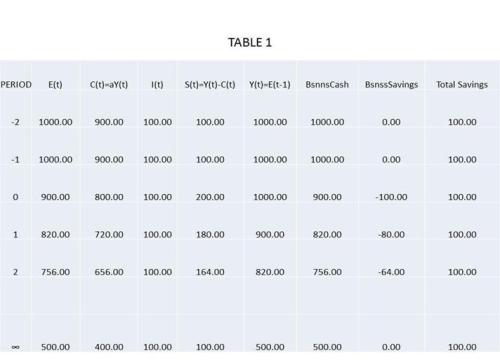
I should have pointed out that if one made the trivial adjustment in the expenditure-income lag, so that incomes earned in one period are not at the end of the current period, but at the beginning of the following period, then income and expenditure and savings and investment would not remain equal over the course of the adjustment from the old to the new equilibrium. The sequence of adjustments under the alternative assumption is shown in Table 1 below.

Of course, if we assume that there is a one-period lag between expenditure and income, one could define something called total savings, which would be household savings plus business savings, where business savings is defined as the difference between cash held by businesses at the end of the current period and cash held by businesses at the end of the previous period. And total savings is identically equal to investment. However, it is important to bear in mind that from the point of view of the simple income-expenditure model, the relevant causal variable in determining equilibrium is not total savings, but household savings.

Why do I say that household savings, not business savings, is the relevant causal factor in determining equilibrium income in the simple income-expenditure model? The reason should be obvious: the solution for equilibrium in the simple income-expenditure model is Y = A/(1 – MPC), where A represents the autonomous component of consumption plus planned investment by business firms and MPC is the marginal propensity to consume by households, so that (1 – MPC) is the marginal propensity to save (MPS) . . . by households!

In this setup, business savings is a pure residual adjusting to make up the difference between household savings and investment. When household savings exceeds investment, businesses accumulate their holdings of cash, and when investment is greater than household saving, businesses reduce their accumulate cash. The operation of the banking system might be relevant at this point, but that analysis would take this discussion to a whole new level, which I am not going to get started on at this point.

I will close at this point by just saying that I think that I have provided an answer to the following comment on my previous post asking what is gained by introducing an alternative set of definitions of saving and investment under which savings and investment are equal only in equilibrium, but not otherwise:

But let’s just say you have a system of accounts where definitions are different and saving is different from investment. I can do a mathematical transformation to a new set of variables in which standard identities hold. What is the point of writing so much? Absolutely nothing.

The point of course is that by defining savings and investment so that they are equal only in equilibrium, we now have a system of two linear equations in two unknowns that can be solved for a unique solution, something that cannot be done if savings and investment are identically equal. Second, when we have defined savings and investment so that they can be unequal, but define their equality to be a condition of equilibrium, we can write the following dynamic relationships characterizing the system:

dY/dt = 0 <=> I = S

dY/dt > 0 <=> I > S

dY/dt < 0 <=> I < S

where I and S are defined under the behavioral assumptions in this example as actual investment by businesses and saving by households. The precise definition of I and S would depend, in each particular case, on the specific behavioral assumptions about the underlying lag structure of the model for that particular case. The definitional equality of total savings and investment has no causal significance, but simply reflects the fact that total savings is defined in such a way that it must equal investment.

The definitional equality of savings and investment, as Scott Sumner has observed, is exactly analogous to the quantity identity MV ≡ PY, when V is treated not as the reciprocal of the amount of money demanded as a fraction of income — which is to say as a measurable magnitude understood to be a function of specifiable independent variables — but simply as a residual whose value, by definition, must always be identically equal to PY/M. The quantity identity, lacking being consistent with all possible states of the world, because V is defined not as an independent variable, but as a mere residual. The quantity identity is therefore of no use in describing the dynamic process of adjustment to a change in the quantity of money or what in telling us what are the causes of such a process.

UPDATE (3/29/15): In writing a response to Jamie’s comment, I realized that in the third paragraph after the table above, I misstated the relationship between business savings and the difference between investment and household savings. I have made the correction, and apologize for not being more careful.

Of Bathtubs, Drains, and Faucets

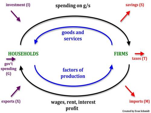
I was planning to write another installment in my series of posts on the savings-investment identity in which I have been working through and summarizing Richard Lipsey’s essay “The Foundations of the Theory of National Income.” Perhaps I will get to my next installment later this week. If not, then I hope to do so early next week. But it occurred to me that the best way to explain why saving is not identical to investment is by framing the discussion in terms of the familiar circular-flow schematic model of income and expenditure. The accompanying diagram is a typical representation of the circular-flow model, with a government sector (government spending and taxes) and a foreign sector (exports and imports) included in addition to just circular_flow_modelinvestment and saving.

As indicated by the arrows in the diagram, investment, government spending, and exports are added to the circular flow while savings, taxes and imports are withdrawn from the circular. In the conventional terminology, investment, government spending and exports are injections, and savings, taxes and imports are leakages. And, of course, a basic property of the model is that injections and leakages are equal. It is only in the simplest model, with no government and with no foreign sector, so that there is just one injection (investment) and one leakage (saving), in which the familiar equality between investment and savings holds.

So the question that I want to ask now is simply this: is the equality in the simple one-sector model between injections (investment) and leakages (savings) an equality that may or may not be true, or is it an identity that must necessarily be satisfied in all places and at all times?

Well, rather than try to argue this through in terms of abstract economic or accounting reasoning, let’s think about it in terms of a simple physical analogy, one that we could actually demonstrate for ourselves in our own homes. So think of a bathtub with some water in it. Depending on the size of the bathtub and the amount of water in the bathtub, the water will reach some uniform height in the bathtub. Let’s call that uniform water level an equilibrium. It’s an equilibrium, because if that’s all the water there is in the bathtub, and we don’t let any water out of the bathtub, and, for purposes of our little thought experiment, we ignore any evaporation, that water level will persist indefinitely, with no tendency to change. No water in, no water out, and you have a constant water level. In other words, with no injections and no leakages, the water level of the bathtub is stable; it does not change. The water level is in equilibrium.

But if you turn on the faucet and water starts to flow into the bathtub, the water level will start to rise. As long as water is being injected into the bathtub, the water level will keep rising, and the water level will not be in equilibrium. However, if you unplug the drain to the bathtub, water will start flowing out of the bathtub. What happens to the water level? That depends on whether water is leaking out of the bathtub through the drain faster than water is being injected into the bath tub through the faucet. If injections are greater than leakages, the water level will rise, and if leakages are greater than injections, the water level will fall. And if, by chance or design, injections are exactly equal to leakages, then the water level will be stable and back in equilibrium. Thus, the condition for a stable water level is that injections be exactly equal to leakages. When injections into, and leakages from, the bathtub are equal, the water level of the bathtub is in equilibrium. When injections are greater than leakages, the water level rises, and when leakages are greater than injections the water level falls.

I think all that is pretty elementary, and I am guessing that if you look in any textbook treatment of injections and leakages in the circular flow of income, you will find a similar story about the effect of a difference between injections and leakages on the level of income. (Check out the Wikipedia article on the circular flow of income, especially the section on equilibrium.)

So, if you believe that investment and savings are identically equal, please tell me whether you also believe that injections and leakages are identically equal. And if you do believe that injections and leakages are identically equal, please explain to me what the difference is between the circular-flow-of-income model with injections and leakages identically equal in equilibrium or out of equilibrium and the bathtub model in which the water level can change only insofar as injections and leakages are not equal.

Why Theories of National Income Based on Accounting Identities Are Nonsensical and Error-Ridden, Part III

In my previous post, I argued that an accounting identity, which tells us that two expressions are defined to be the same, must hold in every state of the world, and therefore could not be disproved by any conceivable observation. So if I define savings and investment (or income and expenditure) to be the same thing, I am simply restricting my semantic description of the world, I am not restricting in any way the set of observable states of the world that conform to my semantic convention. An accounting identity therefore has no empirical content, which means that the accounting identity between savings and investment cannot explain the process by which a macroeconomic model adjusts to a parametric change in the model, traversing from a pre-existing equilibrium with savings and investment being equal to a new equilibrium with savings and investment equal.

In his paper, “The Foundations of the Theory of National Income,” which I am attempting to summarize and explain in this series of posts, R. G. Lipsey provides a numerical example of such an adjustment path. And it will be instructive to follow that path in some detail. The key point about this model is the assumption that households decide how much to save and consume in the current period based on the disposable income received in the previous period. The assumption that all receipts of the business firms are paid out to owners and providers of factor services at the end of each period is a behavioral assumption (not an accounting identity) that rules out any change in the retained earnings held by firms. If firms were accumulating financial assets, then their payments to households would not match their receipts. The following simple model reflects a one-period lag (known as a Robertsonian lag) between household earnings and household consumption.

C(t) = aY(t-1) (behavioral assumption)

I(t) = I* (behavioral assumption)

E(t) ≡ C(t) + I(t) (accounting identity)

Y(t) ≡ C(t) + S(t) (accounting identity)

Y(t) = E(t) (behavioral assumption)

Y(t-1) = Y(t) (equilibrium condition)

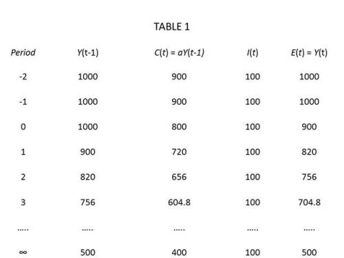
Assume that the economy starts off with a = .9 and I(t) = 100. The system is easily solved for E = Y = 1000, with C = 900 and I = 100. Savings, which is the difference between Y and C, is 100, just equal to I. The definition of saving will have to be fleshed out further below. Now assume that there is a parametric change in a (the marginal propensity to consume) to .8 from .9. This change causes equilibrium income to fall from 1000 to 500. By assumption, investment is constant, so that in the new equilibrium saving remains equal to 100. The change in income is reflected in a drop in consumption from 900 to 400. But given the one-period lag between earnings and expenditure, we can follow how the system changes over time, moving closer and closer to the new equilibrium in each successive period, as shown in the following table.

Consider the following questions.

First, in the course of this period-by-period adjustment, will there be any unplanned investment?

Second, in this example, the parametric change — an increase in the propensity of households to save — may be described as an increase in planned savings by households. Planned investment is unchanged. With planned savings greater than planned investment, will the household plans to increase savings be frustrated (implying positive or negative unplanned savings) as alleged in proposition 3 in the list of erroneous propositions provided earlier in the first installment in this series (see appendix below).

The answer to the first question is: not necessarily. There is nothing to prevent us from assuming that all firms correctly anticipate the reduction in consumer demand, so that production falls along with consumption with no change in inventories. It is not necessary to assume that firms can foresee the future; it could be that all consumption is in the form of services, or that production is undertaken only in response to consumer orders. With inventories unchanged, there is no unplanned investment.

The answer to the second question is that it depends on what is meant by unplanned savings. Unplanned savings could mean that households wind up saving an amount other than the amount that they had intended to save at the beginning of the period; households intended to save 200 at the beginning of period 0, but because their income turned out to be only 900, instead of 1000, in period 0, household savings, under the accounting identity, is only 100 instead of 200. However, households intended to consume 800 in period 0, and that is the amount that they actually consumed. The only sense in which households did not execute their intended plans is that household income in period 0 was less than households had expected. Lipsey calls this a distinction between plans in the point sense, and plans in the schedule sense. In this scenario, while plans in the schedule sense are carried out, plans in the point sense are not, because households do not end up at the point on their consumption functions that they had expected to be on.

So the equilibrium condition above that income does not change from one period to the next can be restated as follows: the system is in equilibrium when planned savings equals realized savings. Planned savings is the unconsumed portion of households’ expected income, which is the income households earned in the previous period. The definition embodies a specific behavioral hypothesis about how households formulate their expectations of income in the future.

S_p_(t) ≡ Y(t-1) – C(t).

Realized savings is the unconsumed portion of households’ actual income in the current period. It can be written as

S_r_(t) ≡ Y(t) – C(t).

Or restated differently yet again, the equilibrium condition is that actual disposable income in period t equals expected disposable income in period t.

Let’s flesh out the behavioral assumptions behind this model in a bit more detail. Business firms disburse income to households (owners and providers of factor services) at the end of each period. Households decide how much to save and consume in the upcoming period after receiving their incomes from firms at the close of the previous period. Savings are in the form of bond purchases made at the start of the period. Based on the consumption and savings plans formulated by households at the start of the new period, firms decide how much output to produce and how much labor to hire to produce that output, firms immediately notifying households how many hours they will work in the upcoming period. However, households are committed to the consumption plans already made at the beginning of the period, so they must execute those plans even if the incomes earned during the period are less than anticipated.

In our example, by choosing to increase their savings to 200 through bond purchases at the beginning of the upcoming period, while reducing consumption from 900 to 800, households cause business firms to reduce output from 1000 to 900 (investment being unchanged), and to reduce employment (measured in terms of total hours worked) by 11.1%. After buying bonds equal to 200, households have 800 left in cash, with which they finance their purchases for the rest of the month. So it is not obvious that households were unable to execute any of their plans  during the period. However, at the end of the period, households receive only 900 in income from business firms, so although households did buy bonds equal to 200 at the start of the period, they carry over only 900 in cash into the next period, not 1000 as expected. Thus, realized savings are only 100 instead of 200, because household cash holding at the endo f the period turned out to be 100 less than expected. Nevertheless, it is difficult to identify any plan to save that was frustrated, inasmuch as households did purchase bonds equal to 200 at the beginning of the period, and did reduce consumption as planned. As Lipsey puts it:

[W]hether or not the actual real plans laid by households are frustrated depends on what plans households lay, i.e., it depends on our behaviour assumption, not on our definitions. If we assume that households make point plans about their bonds, and schedules plans about their transactions and precautionary balances, then no frustration of plans occurs.

If the statement quoted in (3) [see appendix below] is meant to have empirical content, it depends on a very specific hypothesis about households’ savings plans. These plans must be made in the point and not in the schedule sense, and the plans must include not only additions to the stock of income-earning assets, but also point-plans concerning transactions balances even though the household does not now know what level of transactions the balances will be required to facilitate. . . .

[W]e are now in a position to see what is wrong with statement (2), that actual savings must always equal actual investment, and statement (5), which draws the analogy with demand and supply analysis. Consider statement (2) first.

In the General Theory, Keynes stressed the fact that savings and investment decisions are made by different groups and that there is thus, no reason why planned investment should equal planned savings. [It has been argued] that, although plans can differ, actual realised saving must always be equal to actual realised investment, and, therefore, when planned savings does not equal planned investment, either the plans of savers, or of investors, must be frustrated. Of course, it is quite possible to define savings and investment so that they are the same thing, but it is a basic error to equate the magnitude so defined with the magnitude about which savers actually lay plans. Since ex post S and I as defined bear no relation to the magnitudes about which savers actually make plans, we can deduce nothing about what happens when ex ante S is not equal to ex ante I from the fact that we chose to use the terms ex post S and ex post I to refer to a single, and different, magnitude. The basic error arises from the assumption that households and firms make plans about the same magnitude when they are planning their savings and investment. The traditional theory defines investment as goods produced and not sold to households (= capital goods plus changes in inventories). According to our theory of the behaviour of firms, this is what firms do lay plans about: they plan to add so many capital goods and so many inventories to their existing holdings. The theory then says I ≡ S, and , thus, builds in the implicit assumption that households lay plans about the same magnitude. But according to the standard theory of household behaviour, they do not do so! Households, not subject to money illusion, are assumed to wish to lay aside a certain quantity of real purchasing power which is either used to increase the holdings of cash or used to purchase bonds. There is nothing in the standard theory of household behaviour that leads us to hypothesise that households care whether or not there exists – produced but unconsumed – a physical stock of goods which is the counterpart of the money they have laid aside. Indeed why should they? All they are assumed to care about is the potential real purchasing power of their savings, and this depends only on the amount of money saved, the present price level, and the expected future price level.

This is one of the keys to the whole present confusion: households lay plans about a magnitude that is different from the one that firms lay plans about. Firms plan to have produced and unconsumed a certain quantity of goods, while households plan to leave unspent a certain quantity of purchasing power. This means that it is quite possible for planned investment to differ from planned savings and to have both sets of plans fulfilled so that actual, realized investment differs from actual realized savings. [footnote: Now, of course, we mean by realised S and I the realised magnitudes about which firms and households are actually laying plans. This, of course, does not interfere with the statistician saying that realised savings is identical with realised investment since he refers to a different magnitude when he speaks of realised savings.]

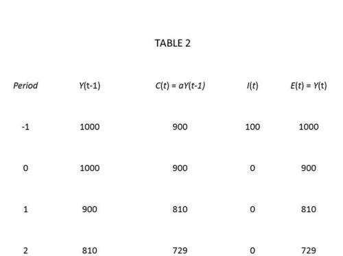
Now consider another variation of the numerical example in Table 1. Instead of a change in the propensity to consume in period 0, assume instead that planned investment drops from 100 to 0. Starting with period -1, Table 2 displays the same initial equilibrium as in Table 1. Because we make a behavioral hypothesis that inventories do not change, planned and realized investment must be zero in period 0 and in all subsequent periods.

According to the national-income identities, savings must equal zero because investment is zero. But what is the actual behavior that corresponds to zero saving? In period 0, households carried over 1000 in cash from period -1. From that 1000, they used 100 to buy bonds and spent the remainder of their disposable incomes on consumption goods. So households planned to save 100 and consume 900, and it appears that they succeeded in executing their plans. But according to the national-income identities, they failed to execute their plan to save 100, and saved only 0, presumably because there were unintended savings of -100 that cancelled out the planned (and executed) savings of 100. So it appears that we have come up against something of a paradox. Here is Lipsey’s solution of the paradox.

[A]ny definitions are possible if consistently used, but this use of the word “unintended” has nothing to do with intended and unintended behaviour. To preserve the identity we must say that the plans of households were frustrated because a real counterpart of the saving they successfully made was not produced. We may say this if we wish, but the danger is that we will think we have said something about the world, and about the actual experiences of households. Indeed, a perusal of established textbooks shows that this confusion has occurred over and over again.

Thus, we conclude that, when we define investment as production not consumed, and savings as income [not consumed] . . . there is no reason why actual savings should not differ from actual investment.

Finally, what about the analogy between savings and investment in macro analysis and demand and supply in micro analysis as in erroneous statement (4) (see appendix)? If we write demand for some good as a function of the price of the good

D = D(p),

and write the supply of some good as a function of the price of the good

S = S(p),

then our equilibrium condition is simply D = S, where D represents desired purchases of the good, and S represents desired sales of the good. Because the act of selling logically entails the activity of purchasing, a purchase and a sale are merely different names for the same thing. So the plans of demanders to buy and the plans of suppliers to sell are plans about the same thing. The plans of demanders to buy and the plans of suppliers to sell cannot be fulfilled simultaneously unless there is an equilibrium in which demand equals supply. The difference between the microeconomic equilibrium in which demand equals supply and the macroeconomic equilibrium in which savings equals investment is that suppliers and demanders in a market are making plans about the same magnitude: sales (aka purchases) of a good. However,

in the national income case the two sets of real plans (savers’ and investors’) are laid about two different magnitudes. Thus the analogy often draw between the two theories in respect of plans and realized quantities is an incorrect one.

Appendix: List of Erroneous Propositions

1 The equilibrium of the basic Keynesian model is given by the intersection of the aggregate demand (i.e., expenditure) function and the 45-degree line representing the accounting identity EY.

2 Although people may try to save different amounts from what people try to invest, savings can’t be different from investment; realized (ex post) savings necessarily always equals realized (ex post) investment.

3 Out of equilibrium, planned savings do not equal planned investment, so it follows from (2) that someone’s plans are being disappointed, and there must be either unplanned savings or dissavings, or unplanned investment or disinvestment

4 The simultaneous fulfilment of the plans of savers and investors occurs only when income is at its equilibrium level just as the plans of buyers and sellers can be simultaneously fulfilled only at the equilibrium price.

5 Whenever savers (households) plan to save an amount different from what investors (business firms) plan to invest, a mechanism operates to ensure that realized savings remain equal to realized investment, despite the attempts of savers and investors to make it otherwise. Indeed, this mechanism is what causes dynamic change in the circular flow of income and expenditure.

6 Since the real world, unlike the simple textbook model, contains a very complex set of interactions, it is not easy to see how savings stay equal to investment even in the worst disequilibrium and the most rapid change.

7 The dynamic behavior of the Keynesian circular flow model in which disequilibrium implies unintended investment or disinvestment can be shown by moving upwards or downwards along the gap between the expenditure function and the 45-degree line in the basic Keynesian model.

Why Theories of National Income Based on Accounting Identities Are Nonsensical and Error-Ridden, Part II

In this installment of my series on Richard Lipsey’s essay “The Foundations of the Theory of National Income,” I am going to focus on a single issue: what inferences about reality are deducible from a definition about the meaning of the terms used in a scientific theory? In my first installment I listed seven common statements about the basic Keynesian income-expenditure model that are found in most textbooks. The first concerned the confusion between the equality of investment and saving (or between income and expenditure) as an equilibrium condition and a definitional identity. Interpreting the equality of savings and investment as an identity essentially means collapsing the entire model onto the 45-degree line and arbitrarily choosing some point on the 45-degree line as the solution of the model.

That nonsensical interpretation of the simple Keynesian cross is obviously unsatisfactory, so, in an effort to save both the definitional identity of savings and investment and the equality of investment and savings as an equilibrium condition, the textbooks have introduced a distinction between ex ante and ex post in which savings and investment are defined to be identically equal ex post, but planned (ex ante) savings may differ from planned (ex ante) investment, their equality being the condition for equilibrium.

Now, to be fair, it is perfectly legitimate to define an equilibrium in terms of plan consistency, and to say that the inconsistency of the plans occasions a process of readjustment in the plans, and that it is the readjustment in the plans which leads to a new equilibrium. The problem with the textbook treatment is that it draws factual inferences about the adjustment process to a disequilibrium in which planned saving is not equal to planned investment from the definitional identity between ex post savings and ex post investment. In particular, the typical textbook treatment infers that in a disequilibrium with planned savings not equal to planned investment, the adjustment process is characterized by unplanned positive or negative investment (inventory accumulation or decumulation) corresponding to the gap between planned savings and planned investment. Identifying a gap between planned saving and planned investment with unplanned inventory accumulation or decumulation, as textbook treatments of the income expenditure model typically do, is logically unfounded.

Again, I want to be careful, I am not saying that unplanned inventory accumulation or decumulation could not occur in response to a difference gap between planned savings and planned investment, or even that such unplanned inventory accumulation or decumulation is unlikely to occur. What I am saying is that the definitional identity between ex post savings and ex post investment does not imply that such inventory accumulation or decumulation takes place and certainly not that the amount by which inventories change is necessarily equal to the gap between planned savings and planned investment.

Richard Lipsey made the key point in his comment on my previous post:

The main issue in this whole discussion is, I think, can we use a definitional identity to rule out an imaginable state of the universe. The answer is “No”, which is why Keynes was wrong. The definitional identity of S ≡ I tells us nothing about what will happen if agents wish to save a different amount from what agents wish to invest.

Here is how Lipsey put it in his 1972 essay:

The error in this interpretation lies in the belief that the identity EY can tell us what can and cannot happen in the world. If it were possible that a definitional identity could rule out certain imaginable events, then such a definitional identity would be an informative statement having empirical content! If it is a genuine definitional identity (which follows from our use of words and is compatible with all states of the universe) then it is only telling us that we are using E and Y to refer to the same thing, and this statement no more allows us to place restrictions on what happens in the world than does the statement that we are not using E and Y to refer to the same thing.

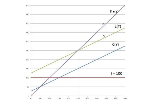
Lipsey illustrated the problem using the simple Keynesian cross diagram. To make the discussion a bit easier to follow, I am going to refer to my own slightly altered version (using a specific numerical example) of the familiar diagram. Setting investment (I) equal to 100 and assuming the following consumption function

C = 25 + .5Y

We can easily solve for an equilibrium income of 250 corresponding to the intersection of the expenditure function with the 45-degree line.

lipsey_45_degreeWhat happens if we posit that the system is at a disequilibrium point, say Y = 400. The usual interpretation is that at Y = 400, planned (ex ante) investment is less than savings and planned (ex ante) expenditure is less than income. Because, actual (ex post) investment is identically equal to savings and because actual (ex post) expenditure is identically equal to income, unplanned investment must occur to guarantee that the investment-savings identity is satisfied. The amount of unplanned investment is shown on the graph as the vertical distance between the expenditure function (E(Y)) at Y = 400 and the 45-degree line at Y = 400. This distance is shown in my diagram as the vertical distance between the points a and b on the diagram, and it is easy to check that the distance corresponds to a value of 75.

So the basic textbook interpretation of the Keynesian cross is using the savings-investment identity to derive a proposition about the behavior of the economy in disequilibrium. It is saying that an economy in disequilibrium with planned investment less than planned savings adjusts to the disequilibrium through unplanned inventory accumulation (unplanned investment) that exactly matches the difference between planned saving and planned investment. But it is logically impossible for a verbal identity (between savings and investment) — an identity that can never be violated in any actual state of the world — to give us any information about what actually happens in the world, because whatever happens in the world, the identity will always be satisfied.

Recall erroneous propositions 2, 3 and 4, listed in part I of this series:

2 Although people may try to save different amounts from what people try to invest, savings can’t be different from investment; realized (ex post) savings necessarily always equals realized (ex post) investment.

3 Out of equilibrium, planned savings do not equal planned investment, so it follows from (2) that someone’s plans are being disappointed, and there must be either unplanned savings or dissavings, or unplanned investment or disinvestment

4 The simultaneous fulfilment of the plans of savers and investors occurs only when income is at its equilibrium level just as the plans of buyers and sellers can be simultaneously fulfilled only at the equilibrium price.

If realized (ex post) savings necessarily always equals realized (ex post) investment, that equality is the result of how we have chosen to define those terms, not because of people actually are behaving, e.g., by unwillingly accumulating inventories or failing to save as much as they had intended to. However people behave, the identity between savings and investment will be satisfied. And whether savers and investors are able to fulfill their plans or are unable to do so cannot possibly be inferred from a definition that says that savings and investment mean the same thing.

In several of his comments on my recent posts, Scott Sumner has cited the professional consensus that savings and investment are defined to be equal. I am not so sure that there is really a consensus on that point, because I don’t think that most economists have thought carefully about what the identity actually means. But even if there is a consensus that savings is identical to investment, no empirical implication follows from that definition. But typical textbook expositions, and I think even Scott himself when he is not being careful, do use the savings-investment identity to make inferences about what actually happens in the real world.

In the next installment, I will go through a numerical example that shows, based on a simple lagged adjustment between consumption and income (household consumption in this period being a function of income in the previous period), that planned savings and planned investment can be realized and unequal in the transition from one equilibrium to another.

PS I apologize for having been unable to respond to a number of comments to previous posts. I will try to respond in the next day or two.


About Me

David Glasner
Washington, DC

I am an economist in the Washington DC area. My research and writing has been mostly on monetary economics and policy and the history of economics. In my book Free Banking and Monetary Reform, I argued for a non-Monetarist non-Keynesian approach to monetary policy, based on a theory of a competitive supply of money. Over the years, I have become increasingly impressed by the similarities between my approach and that of R. G. Hawtrey and hope to bring Hawtrey’s unduly neglected contributions to the attention of a wider audience.

My new book Studies in the History of Monetary Theory: Controversies and Clarifications has been published by Palgrave Macmillan

Follow me on Twitter @david_glasner

Archives

Enter your email address to follow this blog and receive notifications of new posts by email.

Join 3,272 other subscribers
Follow Uneasy Money on WordPress.com