Archive for the 'R. G. Lipsey' Category

Richard Lipsey and the Phillips Curve Redux

Almost three and a half years ago, I published a post about Richard Lipsey’s paper “The Phillips Curve and the Tyranny of an Assumed Unique Macro Equilibrium.” The paper originally presented at the 2013 meeting of the History of Econmics Society has just been published in the Journal of the History of Economic Thought, with a slightly revised title “The Phillips Curve and an Assumed Unique Macroeconomic Equilibrium in Historical Context.” The abstract of the revised published version of the paper is different from the earlier abstract included in my 2013 post. Here is the new abstract.

An early post-WWII debate concerned the most desirable demand and inflationary pressures at which to run the economy. Context was provided by Keynesian theory devoid of a full employment equilibrium and containing its mainly forgotten, but still relevant, microeconomic underpinnings. A major input came with the estimates provided by the original Phillips curve. The debate seemed to be rendered obsolete by the curve’s expectations-augmented version with its natural rate of unemployment, and associated unique equilibrium GDP, as the only values consistent with stable inflation. The current behavior of economies with the successful inflation targeting is inconsistent with this natural-rate view, but is consistent with evolutionary theory in which economies have a wide range of GDP-compatible stable inflation. Now the early post-WWII debates are seen not to be as misguided as they appeared to be when economists came to accept the assumptions implicit in the expectations-augmented Phillips curve.

Publication of Lipsey’s article nicely coincides with Roger Farmer’s new book Prosperity for All which I discussed in my previous post. A key point that Roger makes is that the assumption of a unique equilibrium which underlies modern macroeconomics and the vertical long-run Phillips Curve is neither theoretically compelling nor consistent with the empirical evidence. Lipsey’s article powerfully reinforces those arguments. Access to Lipsey’s article is gated on the JHET website, so in addition to the abstract, I will quote the introduction and a couple of paragraphs from the conclusion.

One important early post-WWII debate, which took place particularly in the UK, concerned the demand and inflationary pressures at which it was best to run the economy. The context for this debate was provided by early Keynesian theory with its absence of a unique full-employment equilibrium and its mainly forgotten, but still relevant, microeconomic underpinnings. The original Phillips Curve was highly relevant to this debate. All this changed, however, with the introduction of the expectations-augmented version of the curve with its natural rate of unemployment, and associated unique equilibrium GDP, as the only values consistent with a stable inflation rate. This new view of the economy found easy acceptance partly because most economists seem to feel deeply in their guts — and their training predisposes them to do so — that the economy must have a unique equilibrium to which market forces inevitably propel it, even if the approach is sometimes, as some believe, painfully slow.

The current behavior of economies with successful inflation targeting is inconsistent with the existence of a unique non-accelerating-inflation rate of unemployment (NAIRU) but is consistent with evolutionary theory in which the economy is constantly evolving in the face of path-dependent, endogenously generated, technological change, and has a wide range of unemployment and GDP over which the inflation rate is stable. This view explains what otherwise seems mysterious in the recent experience of many economies and makes the early post-WWII debates not seem as silly as they appeared to be when economists came to accept the assumption of a perfectly inelastic, long-run Phillips curve located at the unique equilibrium level of unemployment. One thing that stands in the way of accepting this view, however, the tyranny of the generally accepted assumption of a unique, self-sustaining macroeconomic equilibrium.

This paper covers some of the key events in the theory concerning, and the experience of, the economy’s behavior with respect to inflation and unemployment over the post-WWII period. The stage is set by the pressure-of-demand debate in the 1950s and the place that the simple Phillips curve came to play in it. The action begins with the introduction of the expectations-augmented Phillips curve and the acceptance by most Keynesians of its implication of a unique, self-sustaining macro equilibrium. This view seemed not inconsistent with the facts of inflation and unemployment until the mid-1990s, when the successful adoption of inflation targeting made it inconsistent with the facts. An alternative view is proposed, on that is capable of explaining current macro behavior and reinstates the relevance of the early pressure-of-demand debate. (pp. 415-16).

In reviewing the evidence that stable inflation is consistent with a range of unemployment rates, Lipsey generalizes the concept of a unique NAIRU to a non-accelerating-inflation band of unemployment (NAIBU) within which multiple rates of unemployment are consistent with a basically stable expected rate of inflation. In an interesting footnote, Lipsey addresses a possible argument against the relevance of the empirical evidence for policy makers based on the Lucas critique.

Some might raise the Lucas critique here, arguing that one finds the NAIBU in the data because policymakers are credibly concerned only with inflation. As soon as policymakers made use of the NAIBU, the whole unemployment-inflation relation that has been seen since the mid-1990s might change or break. For example, unions, particularly in the European Union, where they are typically more powerful than in North America, might alter their behavior once they became aware that the central bank was actually targeting employment levels directly and appeared to have the power to do so. If so, the Bank would have to establish that its priorities were lexicographically ordered with control of inflation paramount so that any level-of-activity target would be quickly dropped whenever inflation threatened to go outside of the target bands. (pp. 426-27)

I would just mention in this context that in this 2013 post about the Lucas critique, I pointed out that in the paper in which Lucas articulated his critique, he assumed that the only possible source of disequilibrium was a mistake in expected inflation. If everything else is working well, causing inflation expectations to be incorrect will make things worse. But if there are other sources of disequilibrium, it is not clear that incorrect inflation expectations will make things worse; they could make things better. That is a point that Lipsey and Kelvin Lancaster taught the profession in a classic article “The General Theory of Second Best,” 20 years before Lucas published his critique of econometric policy evaluation.

I conclude by quoting Lipsey’s penultimate paragraph (the final paragraph being a quote from Lipsey’s paper on the Phillips Curve from the Blaug and Lloyd volume Famous Figures and Diagrams in Economics which I quoted in full in my 2013 post.

So we seem to have gone full circle from the early Keynesian view in which there was no unique level of GDP to which the economy was inevitably drawn, through a simple Phillips curve with its implied trade-0ff, to an expectations-augmented Phillips curve (or any of its more modern equivalents) with its associated unique level of GDP, and finally back to the early Keynesian view in which policymakers had an option as to the average pressure of aggregate demand at which economic activity could be sustained. However, the modern debated about whether to aim for [the high or low range of stable unemployment rates] is not a debate about inflation versus growth, as it was in the 1950s, but between those who would risk an occasional rise of inflation above the target band as the price of getting unemployment as low as possible and those who would risk letting unemployment fall below that indicated by the lower boundary of the NAIBU  as the price of never risking an acceleration of inflation above the target rate. (p. 427)

JKH on the Keynesian Cross and Accounting Identities

Since beginning this series of posts about accounting identities and their role in the simple Keynesian model, I have received a lot of comments from various commenters, but none has been more persistent, penetrating, and patient in his criticisms than JKH, and I have to say that he has forced me to think very carefully, more carefully than I had ever done before, about my objections to forcing the basic Keynesian model to conform to the standard national income accounting identities. So, although we have not (yet?) reached common ground about how to understand the simple Keynesian model, I can say that my own understanding of how the model works (or doesn’t) is clearer than it was when the series started, so I am grateful to JKH for engaging me in this discussion, even though it has gone on a lot longer than I expected, or really wanted, it to.

In response to my previous post in the series, JKH offered a lengthy critical response. Finding his response difficult to understand and confusing, I wrote a rejoinder that prompted JKH to write a series of further comments. Being preoccupied with a couple of other posts and life in general, I was unable to respond to JKH until now. Given the delay in my response, I decided to respond to JKH in a separate post. I start with JKH’s explanation of how an increase in investment spending is accounted for.

First, the investment injection creates income that accrues to the factors of production – labor and capital. This works through cost accounting. The price at which the investment good is sold covers all costs – including the cost of capital. That said, the price may not cover the theoretical “hurdle rate” for the cost of capital. But that is a technical detail. The equity holders earn some sort of actual residual return, positive or negative. So in the more general sense, the actual cost of capital is accounted for.

So the investment injection creates an equivalent amount of income.

No one says that investment expenditure will not generate an equivalent amount of income; what is questionable is whether the income accrues to factors of production instantaneously. JKH maintains that cost accounting ensures that the accrual is instantaneous, but the recording of a bookkeeping entry is not the same as the receipt of income by households, whose consumption and savings decisions are the key determinant of income adjustments in the Keynesian model. See the tacit assumption in the sentence immediately following.

Consider the effect at the moment the income is fully accrued to the factors of production – before anything else happens.

I understand this to mean that income accrues to factors of production the instant expenditure is booked by the manufacturer of the investment goods; otherwise, I don’t understand why this occurs “before anything else happens.” In a numerical example, JKH posits an increase in investment spending of 100, which triggers added production of 100. For purposes of this discussion, I stipulate that there is no lag between expenditure and output, but I don’t accept that income must accrue to workers and owners of the firm instantaneously as output occurs. Most workers are paid per unit of time, wages being an hourly rate based on the number of hours credited per pay period, and salaries being a fixed amount per pay period. So there is no immediate and direct relationship between worker input into the production process and the remuneration received. The additional production associated with the added investment expenditure and production may or may not be associated with any additional payments to labor depending on how much slack capacity is available to firms and on how the remuneration of workers employed in producing the investment goods is determined.

That amount of income must be saved by the macroeconomy – other things equal. We know this because no new consumer goods or services are produced in this initial standalone scenario of a new investment injection. Therefore, given that saving in the generic sense is income not used to purchase consumer goods and services, this new income created by an assumed investment injection must be saved in the first instance.

Since it is quite conceivable (especially if there is unused capacity available to the firm) that producing new investment goods will not change the total remuneration received by (or owed to) workers in the current period, all additional revenue collected by the firm accruing entirely to the owners of the firm, revenue that might not be included in the next scheduled dividend payment by the firm to shareholders, I am not persuaded that it is unreasonable to assume that there is a lag between expenditure on goods and services and the accrual of income to factors of production. At any rate, whether the firm’s revenue is instantaneously transmuted into household income does not seem to be a question that can be answered in only one way.

What the macroeconomy “must” do is an interesting question, but in the basic Keynesian model, income is earned by households, and it is households, not an abstraction called the macroeconomy, that decide how much to consume and how much to save out of their income. So, in the Keynesian model, regardless of the accounting identities, the relevant saving activity – the saving activity specified by the marginal propensity to save — is the saving of households. That doesn’t mean that the model cannot be extended or reconstructed to allow for saving to be carried out by business firms or by other entities, but that is not how the model, at its most basic level, is set up.

So at this incipient stage before the multiplier process starts, S equals I. That’s before the marginal propensity to consume or save is in motion.

One’s eyes may roll at this point, since the operation of the MPC includes the complementary MPS, and the MPS is a saving function that also operates as the multiplier iterates with successive waves of income creation and consumption.

I understand these two sentences to be an implicit concession that the basic Keynesian model is not being presented in the way it is normally presented in textbooks, a concession that accords with my view that the basic Keynesian model does not always dovetail with the national income identities. Lipsey and I say: don’t impose the accounting identities on the Keynesian model when they are at odds; JKH says reconfigure the basic Keynesian model so that it is consistent with the accounting identities. Where JKH and I may perhaps agree is that the standard textbook story about the adjustment process following a change in spending parameters, in which unintended inventory accumulation corresponding to the frustration of individual plans plays a central role, does not follow from the basic Keynesian model.

So one may ask – how can these apparently opposing ideas be reconciled – the contention that S equals I at a point when the multiplier saving dynamic hasn’t even started?

The investment injection results in an equivalent quantity of income and saving as described earlier. I think you question this off the top while I have claimed it must be the case. But please suspend disbelief for purposes of what I want to describe next, because given that assumed starting point, this should at least reinforce the idea that S = I at all times following that same assumption for the investment injection.

It must be the case, if you define income and expenditure to be identical. If you define them so that they are not identical, which seems both possible and reasonable, then savings and investment are also not identical.

So now assume that the first round of the multiplier math works and there is an initial consumption burst of quantity 66, representing the MPC effect on the income of 100 that was just newly created.

And correspondingly there is new saving of 33.

A pertinent question then is how this gets reflected in income accounting.

As a simplification, assume that the factors of the investment good production who received the new income of 100 are the ones who spend the 66.

So the economy has earned 100 in its factors of investment good production capacity and has now spent 66 in its MPC capacity.

Recall that at the investment injection stage considered on its own, before the multiplier starts to work, the economy saved 100.

Yes, that’s fine if income does accrue simultaneously with expenditure, but that depends on how one chooses to define and measure income, and I don’t feel obligated to adopt the standard accounting definition under all circumstances. (And is it really the case that only one way of defining income is countenanced by accountants?) At any rate, in my first iteration of the lagged model, I specified the lag so that income was earned by households at the end of the period with consumption becoming a function of income in the preceding period. In that setup, the accounting identities were indeed satisfied. However, even with the lag specified that way, the main features of the adjustment process stressed in textbook treatments – frustrated plans, and involuntary inventory accumulation or decumulation – were absent.

Then, in the first stage of the multiplier, the economy spent 66 on consumption. For simplicity of exposition, I’ve assumed those who initially saved were the ones who then spent (I.e. the factors of investment production) But no more income has been assumed to be earned by them. So they have dissaved 66 in the second stage. At the same time, those who produced the 66 of consumer goods have earned 66 as factors of production for those consumer goods. But the consumer goods they produced have been purchased. So there are no remaining consumer goods for them to purchase with their income of 66. And that means they have saved 66.

Therefore, the net saving result of the first round of the multiplier effect is 0.

Thus an MPS of 1/3 has resulted in 0 incremental saving for the macroeconomy. That is because the opening saving of 100 by the factors of production for the investment good has only been redistributed as cumulative saving as between 33 for the investment good production factors and 66 for the consumer good production factors. So the amount of cumulative S still equals the amount of original S, which equals I. And the important observation is that the entire quantity of saving was created originally and at the outset as equivalent to the income earned by the factors of the investment good production.

There is no logical problem here given the definitional imputation of income to households in the initial period before any payments to households have actually been made. However, the model has to be reinterpreted so that household consumption and savings decisions are a function of income earned in the previous period.

Each successive round of the multiplier features a similar combination of equal dissaving and saving.

The result is that cumulative saving remains constant at 100 from the outset and I = S remains in tact always.

The important point is that an original investment injection associated with a Keynesian multiplier process accounts for all the macroeconomic saving to come out of that process, and the MPS fallout of the MPC sequence accounts for none of it.

That is fine, but to get that result, you have to amend the basic Keynesian model or make consumption a function the previous period’s income, which is consistent with what I showed in my first iteration of the lagged model. But that iteration also showed that savings has a somewhat different meaning from the meaning usually attached to the term, saving or dissaving corresponding to a passive accumulation of funds associated with income exceeding or falling short of what it was expected to be in a given period.

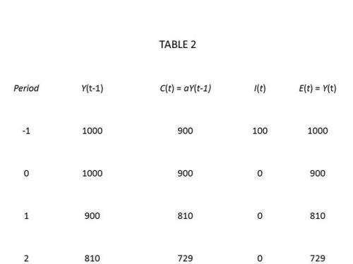
JKH followed up this comment with another one explaining how, within the basic Keynesian model, a change in investment (or in some other expenditure parameter) causes a sequence of adjustments from the old equilibrium to a new equilibrium.

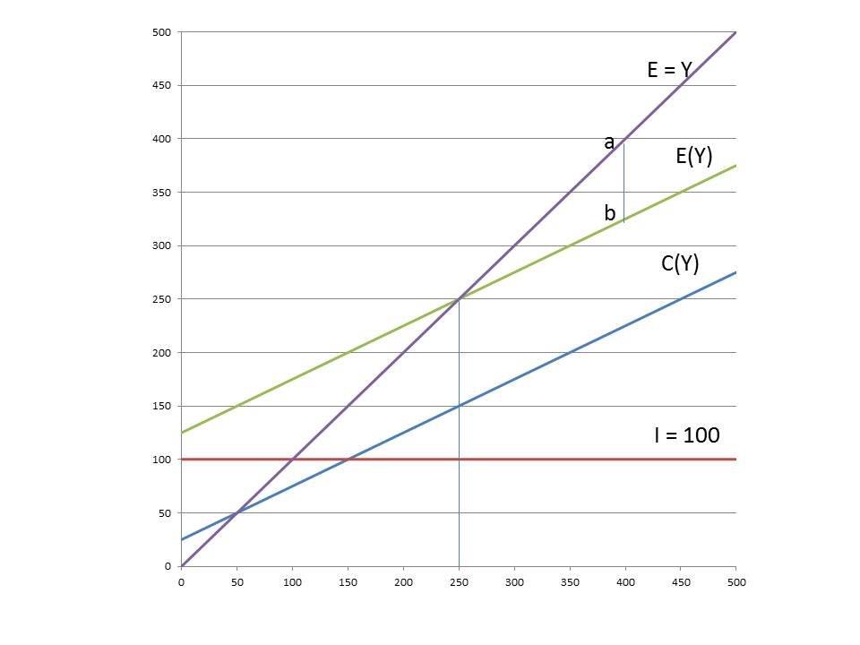
Assume the economy is at an alleged equilibrium point – at the intersection of a planned expenditure line with the 45 degree line.

Suppose planned investment falls by 100. Again, assume MPC = 2/3.

The scenario is one in which investment will be 100 lower than its previous level (bearing in mind we are referring to the level of investment flows here).

Using comparable logic as in my previous comment, that means that both I and S drop by 100 at the outset. There is that much less investment injected and saving created as a result of the economy not operating at a counterfactual level of activity equal to its previous pace.

So expenditure drops by 100 – and that considered just on its own can be represented by a direct vertical drop from the previous equilibrium point down to the planning line.

But as I have said before, such a point is unrealizable in fact, because it lies off the 45 degree line. And that corresponds to the fact that I of 100 generates S of 100 (or in this case a decline in I from previous levels means a decline in S from previous levels). So what happens is that instead of landing on that 100 vertical drop down point, the economy combines (in measured effect) that move with a second move horizontally to the left, where it lands on the 45 degree line at a point where both E and Y have declined by 100. This simply reflects the fact that I = S at all times as described in my previous comment (which again I realize is a contentious supposition for purposes of the broader discussion).

Actually, it is clear that being off the 45-degree line is not a matter of possibility in any causal or behavioral sense, but is simply a matter of how income and expenditure are defined. With income and expenditure suitably defined, income need not equal expenditure. As just shown, if one wants to define income and expenditure so that they are equal at all times, a temporal adjustment process can be derived if current consumption is made a function of income in the previous period (presumably with an implicit behavioral assumption that households expect to earn the same income in the current period that they earned in the previous period). The adjustment can be easily portrayed in the familiar Keynesian cross, provided that the lag is incorporated into the diagram by measuring E(t) on the vertical axis and measures Y(t-1) on the horizontal axis. The 45-degree line then represents the equilibrium condition that E(t) = Y(t-1), which implies (given the implicit behavioral assumption) that actual income equals expected income or that income is unchanged period to period. Obviously, in this setup, the economy can be off the 45-degree line. Following a change in investment, an adjustment process moves from the old expenditure line to the new one continuing in stepwise fashion from the new expenditure line to the 45-degree line and back in successive periods converging on the point of intersection between the new expenditure line and the 45-degree line.

This happens in steps representable by discrete accounting. Common sense suggests that a “plan” can consist of a series of such discrete steps – in which case there is a ratcheting of reduced investment injections down the 45 degree line – or a plan can consist of a single discrete step depending on the scale or on the preference for stepwise analysis. The single discrete step is the clearest way to analyse the accounting record for the economics.

There is no such “plan” in the model, because no one foresees where the adjustment is leading; households assume in each period that their income will be what it was in the previous period, and firms produce exactly what consumers demand without change in inventories. However, all expenditure planned at the beginning of each period is executed (every household remaining on its planned expenditure curve), but households wind up earning less than expected in each period. Suitably amended, I consider this statement to be consistent with Lipsey’s critique of standard textbook expositions of the Keynesian cross adjustment process wherein the adjustment to a new equilibrium is driven by the frustration of plans.

Finally, some brief responses to JKH’s comments on handling lags.

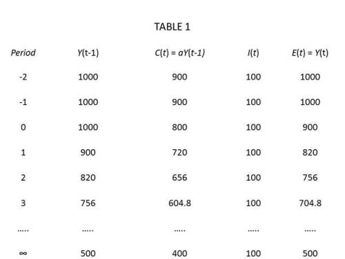
I’m going to refer to standard accounting for Y as Y and the methodology used in the post as LGY (i.e. “Lipsey – Glasner income” ).

Then:

E ( t ) = Y ( t )

E ( t ) = LGY ( t +1)

Standard accounting recognizes income in the time period in which it is earned.

LGY accounting recognizes income in the time period in which it is paid in cash.

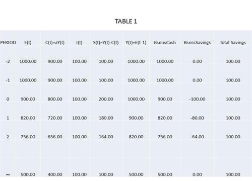
Consider the point in table 1 where the MPC propensity factor drops from .9 to .8. . . .

In the first iteration, E is 900 ( 100 I + 800 C ) but LGY is 1000.

Household saving is shown to be 200.

Here is how standard accounting handles that:

First, a real world example. Suppose a US corporation listed on a stock exchange reports its financial results at the end of each calendar quarter. And suppose it pays its employees once a month. But for each month’s work it pays them at the start of the next month.

Then there is no way that this corporation would report it’s December 31 financial results without showing a liability on its balance sheet for the employee compensation earned in December but not yet paid by December 31. . . .

In effect, the employees have loaned the corporation one months salary until that loan is repaid in the next accounting period.

The corporation will properly list a liability on its balance sheet for wages not yet paid. This may be a “loan in effect,” but employees don’t receive an IOU for the unpaid wages because the wages are not yet due. I am no tax expert, but I am guessing that a liability to pay taxes on the wages owed to, but not yet received by, employees is incurred until the wages are paid, notwithstanding whatever liability is recorded on the books of the corporation. A worker employed in 2014, but not paid until 2015, will owe taxes on his 2015, not 2014, tax return. A “loan in effect” is not the same as an actual payment.

This is precisely what is happening at the macro level in the LGY lag example.

So the standard national income accounting would show E = Y = 900, with a business liability of 900 at the end of the period. Households would have a corresponding financial asset of 900.

The “financial asset” in question is a fiction. There is a claim, but the claim at the end of the period has not fallen due, so it represents a claim to an expected future payment. I expect to get a royalty check next month, for copies of my book sold last year. I don’t consider that I have received income until the check arrives from my publisher, regardless of how the publisher chooses to record its liability to me on its books. And I will not pay any tax on books sold in 2014 until 2016 when I file my 2015 tax return. And I certainly did not consider the expected royalties as income last year when the books were sold. In fact, I don’t know — and never will — when in 2014 the books were sold.

Back at the beginning of that same period, business repaid the prior period liability of 1000 to households. But they received cash revenue of 900 during the period. So as the post says, business cash would have declined by 100 during the period.

This component of 100 when received by households is part of a loan repayment in effect. This does not constitute a component of standard income accounting Y or S for households. This sort of thing is captured In flow of funds accounting.

Just as LGY is the delayed payment of Y earned in the previous period, LGS overstates S by the difference between LGY and Y.

For example, when E is 900, LGY is 1000 and Y is 900. LGS is 200 while S is 100.

So under regular accounting, this systematic LG overstatement reflects the cash repayment of a loan – not the differential receipt of income and saving.

That is certainly a possible interpretation of the assumptions being made, but obviously there are alternative interpretations that are completely consistent with workings of the basic Keynesian model.

And another way of describing this is that households earn Y of 900 and get paid in the same period in the form of a non-cash financial asset of 900, which is in effect a loan to business for the amount of cash that business owes to households for the income the latter have already earned. That loan is repaid in the next period.

Again, I observe that “payments in effect” are being created to avoid working with and measuring actual payments as they take place. I have no problem with such “payments in effect,” but that does not mean that the the magnitudes of interest can be measured in only one way.

There are several ironies in the comparison of LG accounting with standard accounting.

First, using standard accounting in no way impedes the analysis of cash flow lags. In fact, this is the reason for separate balance sheet and flow of funds accounting – so as not to conflate cash flow analysis with the earning of income when there are clear separations between the earning of income and the cash payments to the recipients of that income. The 3 part framework is precise in its treatment of such situations.

Not sure where the irony is. In any event, I don’t see how the 3 part framework adds anything to our understanding of the Keynesian model.

Second, in the scenario constructed for the post, there is no logical connection between a delayed income payment of 1000 and a decision to ramp down consumption propensity. Why would one choose to consume less because an income payment is systematically late? If that was the case, one would ramp down consumption every time a payment was delayed. But every such payment is delayed in this model. Changes in consumption propensity cannot logically be a systematic function of a systematic lag – or consumption propensity would systematically approach 0, which is obviously nonsensical.

This seems to be a misunderstanding of what I wrote. I never suggested that the lag between expenditure and income is connected (logically or otherwise) to the reduction in the marginal propensity to consume. A lag is necessary for there to be a sequential rather than an instantaneous adjustment process to a parameter change in the model, such as a reduced marginal propensity to consume. There is no other connection.

Third, my earlier example of a corporation that delayed an income payment from December until January is a stretch on reality. Corporations have no valid reason to play such cash management games that span accounting periods. They must account for legitimate liabilities that are outstanding when proceeding to the next accounting period.

I never suggested that corporations are playing a game. Wage payments, royalty and dividend payments are made according to fixed schedules, which may not coincide with the relevant time period for measuring economic activity. Fiscal years and calendar years do not always coincide.

Shorter term intra period lags may still exist – as within a one month income payment cycle. But again, so what? There cannot be systemic behavior to reduce consumption propensity due to systematic lags. Moreover, a lot of people get paid every 2 weeks. But that is not even the relevant point. Standard accounting handles any of these issues even at the level of internal management accounting accruals between external financial reporting dates.

I never suggested that the propensity to consume is related to the lag structure in the model. The propensity to consume determines the equilibrium; the lag structure determines the sequence of adjustments, following a change in a spending parameter, from one equilibrium to another.

PS I apologize for this excessively long — even by my long-winded and verbose standards — post.

Why Theories of National Income Based on Accounting Identities Are Nonsensical and Error-Ridden, Part IV

In my previous post, I tried to relate the discussion of accounting identities to the familiar circular-flow diagram with injections into and leakages out of the flows of income, expenditure and output. My hopes that framing the discussion in terms of injections and leakages, with investment viewed as an injection into, and savings as a withdrawal out of, the flows of income and expenditure would help clarify my position about accounting identities were disappointed, as defenders of those accounting identities were highly critical of the injections-leakages analogy, launching a barrage of criticism at my argument that the basic macroeconomic model of income determination should not be understood in terms of the income-expenditure or the investment-savings identities.

I think that criticism of the injections-leakages analogy was, for the most part, misplaced and a based on a misunderstanding of what I have been aiming to do, but much of the criticism was prompted by my incomplete or inadequate explanation of my reasoning. So, before continuing with my summary of Lipsey’s essay on the subject, on which this series is based, I need to address at least some of the points that have been made by my (and Lipsey’s) various critics. In the course of doing so, I believe it will be helpful if I offer a revised version of Lipsey’s Table 1, which I reproduced in part III of this series.

First, I am not saying that the standard accounting identities are wrong. Definitions are neither right nor wrong, but they may be useful or not useful depending on the context. In everyday conversation, we routinely ascribe one of many possible meanings to particular words used by selecting one of the many possible definitions as that which is most likely to make an entire sequence of words – a phrase, a clause, or a sentence – meaningful. Our choice of which definition to use is generally determined by the context in which the word appears. Choosing one definition over another doesn’t mean that others are not valid, just that the others would not work as well or at all in the context in which the word in question appears. Working with an inappropriate definition in a given context can lead, as we all know from personal experience, to confusion, misunderstanding and error. Defining savings and investment to be equal in every state of the world is certainly possible, and doing so is not invalid, but doing so is not necessarily useful in the context of formulating a macroeconomic theory of income determination.

There are two reasons why defining savings and investment to be identically equal in all states of the world is not useful in a macroeconomic theory of income. First, if we define savings and investment (or income and expenditure) to be identically equal, we can’t solve, either algebraically or graphically, the system of equations describing the model for a unique equilibrium. According to the model, aggregate expenditure is assumed to be a function of income, but if income and expenditure are identical, expenditure is simply identical to itself, so the system of equations described by the model collapses onto the 45-degree line representing the expenditure-income identity.

Second, even if we interpret the equality of income and expenditure as an ex ante equilibrium condition, while asserting that identity between income and expenditure must always hold ex post, the ex post definitional equality tells us nothing about the adjustment process that restores equilibrium when, owing to some parameter change that disturbs a pre-existing equilibrium, the ex ante equilibrium condition does not hold. For a dynamic adjustment path to take the model from one equilibrium to another via a sequence of discrete adjustments, the model must incorporate some lags. Without lags, the adjustment would be instantaneous, and the model would move from its old equilibrium to a new equilibrium in one fell swoop. But in the course of a sequence of partial adjustments, savings and investment will typically have to be defined by the model so that they are not equal, and this will be reflected in the implied course of savings and investment if the model is worked out period-by-period. Or if you were to observe the Phillips machine (a hydraulic macroeconomic model built by A. W. Phillips of Phillips Curve fame) in action, you could actually see that the savings and investment flows were of unequal magnitudes as machine responded to a change in the settings and moved from one hydraulic equilibrium to another.

It is a common mistake, and the primary object of Richard Lipsey’s scorn in his essay, to attribute causal significance to the savings-investment identity, as if it were the force of the identity itself that guided the dynamic adjustment, when, in reality, the identity, which can always be recovered if one does all the necessary accounting and classifies all the transactions according to the accounting conventions, is irrelevant to the adjustment path. Doing the accounting does not explain how the model moves from the old to a new equilibrium; it just assures us that nothing has been omitted from a final description of what has happened. Rather, the causal mechanism driving the adjustment process can be described using the intuitive idea that income changes because there are injections (in the form of investment) into the income and expenditure flows and leakages (in the form of savings) out of those flows, and when the injections and leakages are unequal in magnitude, the discrepancy between the injections and the leakages causes a corresponding change in the income and expenditure flows.

One commenter pointed out that, even in the numerical example (taken from Lipsey’s essay) that I gave in my earlier post, the sequence of adjustments preserved the definitional equality between savings and investment and income and expenditure, even though the verbal explanation of the adjustment process showed that the equality of savings and investment required a rather forced interpretation of the meaning of savings: the difference between the cash balance expected at the end of a period and the actual cash balance at the end of the period. This peculiar interpretation of savings and its equality with investment reflected the way that Lipsey chose to introduce a lag between expenditure and income into the model: by assuming that income was disbursed by businesses to households at the end of the period in which households provide services to businesses. The income received at the end of one period is then used to finance consumption expenditures and savings in the following period.

I should have pointed out that if one made the trivial adjustment in the expenditure-income lag, so that incomes earned in one period are not at the end of the current period, but at the beginning of the following period, then income and expenditure and savings and investment would not remain equal over the course of the adjustment from the old to the new equilibrium. The sequence of adjustments under the alternative assumption is shown in Table 1 below.

Of course, if we assume that there is a one-period lag between expenditure and income, one could define something called total savings, which would be household savings plus business savings, where business savings is defined as the difference between cash held by businesses at the end of the current period and cash held by businesses at the end of the previous period. And total savings is identically equal to investment. However, it is important to bear in mind that from the point of view of the simple income-expenditure model, the relevant causal variable in determining equilibrium is not total savings, but household savings.

Why do I say that household savings, not business savings, is the relevant causal factor in determining equilibrium income in the simple income-expenditure model? The reason should be obvious: the solution for equilibrium in the simple income-expenditure model is Y = A/(1 – MPC), where A represents the autonomous component of consumption plus planned investment by business firms and MPC is the marginal propensity to consume by households, so that (1 – MPC) is the marginal propensity to save (MPS) . . . by households!

In this setup, business savings is a pure residual adjusting to make up the difference between household savings and investment. When household savings exceeds investment, businesses accumulate their holdings of cash, and when investment is greater than household saving, businesses reduce their accumulate cash. The operation of the banking system might be relevant at this point, but that analysis would take this discussion to a whole new level, which I am not going to get started on at this point.

I will close at this point by just saying that I think that I have provided an answer to the following comment on my previous post asking what is gained by introducing an alternative set of definitions of saving and investment under which savings and investment are equal only in equilibrium, but not otherwise:

But let’s just say you have a system of accounts where definitions are different and saving is different from investment. I can do a mathematical transformation to a new set of variables in which standard identities hold. What is the point of writing so much? Absolutely nothing.

The point of course is that by defining savings and investment so that they are equal only in equilibrium, we now have a system of two linear equations in two unknowns that can be solved for a unique solution, something that cannot be done if savings and investment are identically equal. Second, when we have defined savings and investment so that they can be unequal, but define their equality to be a condition of equilibrium, we can write the following dynamic relationships characterizing the system:

dY/dt = 0 <=> I = S

dY/dt > 0 <=> I > S

dY/dt < 0 <=> I < S

where I and S are defined under the behavioral assumptions in this example as actual investment by businesses and saving by households. The precise definition of I and S would depend, in each particular case, on the specific behavioral assumptions about the underlying lag structure of the model for that particular case. The definitional equality of total savings and investment has no causal significance, but simply reflects the fact that total savings is defined in such a way that it must equal investment.

The definitional equality of savings and investment, as Scott Sumner has observed, is exactly analogous to the quantity identity MV ≡ PY, when V is treated not as the reciprocal of the amount of money demanded as a fraction of income — which is to say as a measurable magnitude understood to be a function of specifiable independent variables — but simply as a residual whose value, by definition, must always be identically equal to PY/M. The quantity identity, lacking being consistent with all possible states of the world, because V is defined not as an independent variable, but as a mere residual. The quantity identity is therefore of no use in describing the dynamic process of adjustment to a change in the quantity of money or what in telling us what are the causes of such a process.

UPDATE (3/29/15): In writing a response to Jamie’s comment, I realized that in the third paragraph after the table above, I misstated the relationship between business savings and the difference between investment and household savings. I have made the correction, and apologize for not being more careful.

Why Theories of National Income Based on Accounting Identities Are Nonsensical and Error-Ridden, Part III

In my previous post, I argued that an accounting identity, which tells us that two expressions are defined to be the same, must hold in every state of the world, and therefore could not be disproved by any conceivable observation. So if I define savings and investment (or income and expenditure) to be the same thing, I am simply restricting my semantic description of the world, I am not restricting in any way the set of observable states of the world that conform to my semantic convention. An accounting identity therefore has no empirical content, which means that the accounting identity between savings and investment cannot explain the process by which a macroeconomic model adjusts to a parametric change in the model, traversing from a pre-existing equilibrium with savings and investment being equal to a new equilibrium with savings and investment equal.

In his paper, “The Foundations of the Theory of National Income,” which I am attempting to summarize and explain in this series of posts, R. G. Lipsey provides a numerical example of such an adjustment path. And it will be instructive to follow that path in some detail. The key point about this model is the assumption that households decide how much to save and consume in the current period based on the disposable income received in the previous period. The assumption that all receipts of the business firms are paid out to owners and providers of factor services at the end of each period is a behavioral assumption (not an accounting identity) that rules out any change in the retained earnings held by firms. If firms were accumulating financial assets, then their payments to households would not match their receipts. The following simple model reflects a one-period lag (known as a Robertsonian lag) between household earnings and household consumption.

C(t) = aY(t-1) (behavioral assumption)

I(t) = I* (behavioral assumption)

E(t) ≡ C(t) + I(t) (accounting identity)

Y(t) ≡ C(t) + S(t) (accounting identity)

Y(t) = E(t) (behavioral assumption)

Y(t-1) = Y(t) (equilibrium condition)

Assume that the economy starts off with a = .9 and I(t) = 100. The system is easily solved for E = Y = 1000, with C = 900 and I = 100. Savings, which is the difference between Y and C, is 100, just equal to I. The definition of saving will have to be fleshed out further below. Now assume that there is a parametric change in a (the marginal propensity to consume) to .8 from .9. This change causes equilibrium income to fall from 1000 to 500. By assumption, investment is constant, so that in the new equilibrium saving remains equal to 100. The change in income is reflected in a drop in consumption from 900 to 400. But given the one-period lag between earnings and expenditure, we can follow how the system changes over time, moving closer and closer to the new equilibrium in each successive period, as shown in the following table.

Consider the following questions.

First, in the course of this period-by-period adjustment, will there be any unplanned investment?

Second, in this example, the parametric change — an increase in the propensity of households to save — may be described as an increase in planned savings by households. Planned investment is unchanged. With planned savings greater than planned investment, will the household plans to increase savings be frustrated (implying positive or negative unplanned savings) as alleged in proposition 3 in the list of erroneous propositions provided earlier in the first installment in this series (see appendix below).

The answer to the first question is: not necessarily. There is nothing to prevent us from assuming that all firms correctly anticipate the reduction in consumer demand, so that production falls along with consumption with no change in inventories. It is not necessary to assume that firms can foresee the future; it could be that all consumption is in the form of services, or that production is undertaken only in response to consumer orders. With inventories unchanged, there is no unplanned investment.

The answer to the second question is that it depends on what is meant by unplanned savings. Unplanned savings could mean that households wind up saving an amount other than the amount that they had intended to save at the beginning of the period; households intended to save 200 at the beginning of period 0, but because their income turned out to be only 900, instead of 1000, in period 0, household savings, under the accounting identity, is only 100 instead of 200. However, households intended to consume 800 in period 0, and that is the amount that they actually consumed. The only sense in which households did not execute their intended plans is that household income in period 0 was less than households had expected. Lipsey calls this a distinction between plans in the point sense, and plans in the schedule sense. In this scenario, while plans in the schedule sense are carried out, plans in the point sense are not, because households do not end up at the point on their consumption functions that they had expected to be on.

So the equilibrium condition above that income does not change from one period to the next can be restated as follows: the system is in equilibrium when planned savings equals realized savings. Planned savings is the unconsumed portion of households’ expected income, which is the income households earned in the previous period. The definition embodies a specific behavioral hypothesis about how households formulate their expectations of income in the future.

S_p_(t) ≡ Y(t-1) – C(t).

Realized savings is the unconsumed portion of households’ actual income in the current period. It can be written as

S_r_(t) ≡ Y(t) – C(t).

Or restated differently yet again, the equilibrium condition is that actual disposable income in period t equals expected disposable income in period t.

Let’s flesh out the behavioral assumptions behind this model in a bit more detail. Business firms disburse income to households (owners and providers of factor services) at the end of each period. Households decide how much to save and consume in the upcoming period after receiving their incomes from firms at the close of the previous period. Savings are in the form of bond purchases made at the start of the period. Based on the consumption and savings plans formulated by households at the start of the new period, firms decide how much output to produce and how much labor to hire to produce that output, firms immediately notifying households how many hours they will work in the upcoming period. However, households are committed to the consumption plans already made at the beginning of the period, so they must execute those plans even if the incomes earned during the period are less than anticipated.

In our example, by choosing to increase their savings to 200 through bond purchases at the beginning of the upcoming period, while reducing consumption from 900 to 800, households cause business firms to reduce output from 1000 to 900 (investment being unchanged), and to reduce employment (measured in terms of total hours worked) by 11.1%. After buying bonds equal to 200, households have 800 left in cash, with which they finance their purchases for the rest of the month. So it is not obvious that households were unable to execute any of their plans  during the period. However, at the end of the period, households receive only 900 in income from business firms, so although households did buy bonds equal to 200 at the start of the period, they carry over only 900 in cash into the next period, not 1000 as expected. Thus, realized savings are only 100 instead of 200, because household cash holding at the endo f the period turned out to be 100 less than expected. Nevertheless, it is difficult to identify any plan to save that was frustrated, inasmuch as households did purchase bonds equal to 200 at the beginning of the period, and did reduce consumption as planned. As Lipsey puts it:

[W]hether or not the actual real plans laid by households are frustrated depends on what plans households lay, i.e., it depends on our behaviour assumption, not on our definitions. If we assume that households make point plans about their bonds, and schedules plans about their transactions and precautionary balances, then no frustration of plans occurs.

If the statement quoted in (3) [see appendix below] is meant to have empirical content, it depends on a very specific hypothesis about households’ savings plans. These plans must be made in the point and not in the schedule sense, and the plans must include not only additions to the stock of income-earning assets, but also point-plans concerning transactions balances even though the household does not now know what level of transactions the balances will be required to facilitate. . . .

[W]e are now in a position to see what is wrong with statement (2), that actual savings must always equal actual investment, and statement (5), which draws the analogy with demand and supply analysis. Consider statement (2) first.

In the General Theory, Keynes stressed the fact that savings and investment decisions are made by different groups and that there is thus, no reason why planned investment should equal planned savings. [It has been argued] that, although plans can differ, actual realised saving must always be equal to actual realised investment, and, therefore, when planned savings does not equal planned investment, either the plans of savers, or of investors, must be frustrated. Of course, it is quite possible to define savings and investment so that they are the same thing, but it is a basic error to equate the magnitude so defined with the magnitude about which savers actually lay plans. Since ex post S and I as defined bear no relation to the magnitudes about which savers actually make plans, we can deduce nothing about what happens when ex ante S is not equal to ex ante I from the fact that we chose to use the terms ex post S and ex post I to refer to a single, and different, magnitude. The basic error arises from the assumption that households and firms make plans about the same magnitude when they are planning their savings and investment. The traditional theory defines investment as goods produced and not sold to households (= capital goods plus changes in inventories). According to our theory of the behaviour of firms, this is what firms do lay plans about: they plan to add so many capital goods and so many inventories to their existing holdings. The theory then says I ≡ S, and , thus, builds in the implicit assumption that households lay plans about the same magnitude. But according to the standard theory of household behaviour, they do not do so! Households, not subject to money illusion, are assumed to wish to lay aside a certain quantity of real purchasing power which is either used to increase the holdings of cash or used to purchase bonds. There is nothing in the standard theory of household behaviour that leads us to hypothesise that households care whether or not there exists – produced but unconsumed – a physical stock of goods which is the counterpart of the money they have laid aside. Indeed why should they? All they are assumed to care about is the potential real purchasing power of their savings, and this depends only on the amount of money saved, the present price level, and the expected future price level.

This is one of the keys to the whole present confusion: households lay plans about a magnitude that is different from the one that firms lay plans about. Firms plan to have produced and unconsumed a certain quantity of goods, while households plan to leave unspent a certain quantity of purchasing power. This means that it is quite possible for planned investment to differ from planned savings and to have both sets of plans fulfilled so that actual, realized investment differs from actual realized savings. [footnote: Now, of course, we mean by realised S and I the realised magnitudes about which firms and households are actually laying plans. This, of course, does not interfere with the statistician saying that realised savings is identical with realised investment since he refers to a different magnitude when he speaks of realised savings.]

Now consider another variation of the numerical example in Table 1. Instead of a change in the propensity to consume in period 0, assume instead that planned investment drops from 100 to 0. Starting with period -1, Table 2 displays the same initial equilibrium as in Table 1. Because we make a behavioral hypothesis that inventories do not change, planned and realized investment must be zero in period 0 and in all subsequent periods.

According to the national-income identities, savings must equal zero because investment is zero. But what is the actual behavior that corresponds to zero saving? In period 0, households carried over 1000 in cash from period -1. From that 1000, they used 100 to buy bonds and spent the remainder of their disposable incomes on consumption goods. So households planned to save 100 and consume 900, and it appears that they succeeded in executing their plans. But according to the national-income identities, they failed to execute their plan to save 100, and saved only 0, presumably because there were unintended savings of -100 that cancelled out the planned (and executed) savings of 100. So it appears that we have come up against something of a paradox. Here is Lipsey’s solution of the paradox.

[A]ny definitions are possible if consistently used, but this use of the word “unintended” has nothing to do with intended and unintended behaviour. To preserve the identity we must say that the plans of households were frustrated because a real counterpart of the saving they successfully made was not produced. We may say this if we wish, but the danger is that we will think we have said something about the world, and about the actual experiences of households. Indeed, a perusal of established textbooks shows that this confusion has occurred over and over again.

Thus, we conclude that, when we define investment as production not consumed, and savings as income [not consumed] . . . there is no reason why actual savings should not differ from actual investment.

Finally, what about the analogy between savings and investment in macro analysis and demand and supply in micro analysis as in erroneous statement (4) (see appendix)? If we write demand for some good as a function of the price of the good

D = D(p),

and write the supply of some good as a function of the price of the good

S = S(p),

then our equilibrium condition is simply D = S, where D represents desired purchases of the good, and S represents desired sales of the good. Because the act of selling logically entails the activity of purchasing, a purchase and a sale are merely different names for the same thing. So the plans of demanders to buy and the plans of suppliers to sell are plans about the same thing. The plans of demanders to buy and the plans of suppliers to sell cannot be fulfilled simultaneously unless there is an equilibrium in which demand equals supply. The difference between the microeconomic equilibrium in which demand equals supply and the macroeconomic equilibrium in which savings equals investment is that suppliers and demanders in a market are making plans about the same magnitude: sales (aka purchases) of a good. However,

in the national income case the two sets of real plans (savers’ and investors’) are laid about two different magnitudes. Thus the analogy often draw between the two theories in respect of plans and realized quantities is an incorrect one.

Appendix: List of Erroneous Propositions

1 The equilibrium of the basic Keynesian model is given by the intersection of the aggregate demand (i.e., expenditure) function and the 45-degree line representing the accounting identity EY.

2 Although people may try to save different amounts from what people try to invest, savings can’t be different from investment; realized (ex post) savings necessarily always equals realized (ex post) investment.

3 Out of equilibrium, planned savings do not equal planned investment, so it follows from (2) that someone’s plans are being disappointed, and there must be either unplanned savings or dissavings, or unplanned investment or disinvestment

4 The simultaneous fulfilment of the plans of savers and investors occurs only when income is at its equilibrium level just as the plans of buyers and sellers can be simultaneously fulfilled only at the equilibrium price.

5 Whenever savers (households) plan to save an amount different from what investors (business firms) plan to invest, a mechanism operates to ensure that realized savings remain equal to realized investment, despite the attempts of savers and investors to make it otherwise. Indeed, this mechanism is what causes dynamic change in the circular flow of income and expenditure.

6 Since the real world, unlike the simple textbook model, contains a very complex set of interactions, it is not easy to see how savings stay equal to investment even in the worst disequilibrium and the most rapid change.

7 The dynamic behavior of the Keynesian circular flow model in which disequilibrium implies unintended investment or disinvestment can be shown by moving upwards or downwards along the gap between the expenditure function and the 45-degree line in the basic Keynesian model.

Why Theories of National Income Based on Accounting Identities Are Nonsensical and Error-Ridden, Part II

In this installment of my series on Richard Lipsey’s essay “The Foundations of the Theory of National Income,” I am going to focus on a single issue: what inferences about reality are deducible from a definition about the meaning of the terms used in a scientific theory? In my first installment I listed seven common statements about the basic Keynesian income-expenditure model that are found in most textbooks. The first concerned the confusion between the equality of investment and saving (or between income and expenditure) as an equilibrium condition and a definitional identity. Interpreting the equality of savings and investment as an identity essentially means collapsing the entire model onto the 45-degree line and arbitrarily choosing some point on the 45-degree line as the solution of the model.

That nonsensical interpretation of the simple Keynesian cross is obviously unsatisfactory, so, in an effort to save both the definitional identity of savings and investment and the equality of investment and savings as an equilibrium condition, the textbooks have introduced a distinction between ex ante and ex post in which savings and investment are defined to be identically equal ex post, but planned (ex ante) savings may differ from planned (ex ante) investment, their equality being the condition for equilibrium.

Now, to be fair, it is perfectly legitimate to define an equilibrium in terms of plan consistency, and to say that the inconsistency of the plans occasions a process of readjustment in the plans, and that it is the readjustment in the plans which leads to a new equilibrium. The problem with the textbook treatment is that it draws factual inferences about the adjustment process to a disequilibrium in which planned saving is not equal to planned investment from the definitional identity between ex post savings and ex post investment. In particular, the typical textbook treatment infers that in a disequilibrium with planned savings not equal to planned investment, the adjustment process is characterized by unplanned positive or negative investment (inventory accumulation or decumulation) corresponding to the gap between planned savings and planned investment. Identifying a gap between planned saving and planned investment with unplanned inventory accumulation or decumulation, as textbook treatments of the income expenditure model typically do, is logically unfounded.

Again, I want to be careful, I am not saying that unplanned inventory accumulation or decumulation could not occur in response to a difference gap between planned savings and planned investment, or even that such unplanned inventory accumulation or decumulation is unlikely to occur. What I am saying is that the definitional identity between ex post savings and ex post investment does not imply that such inventory accumulation or decumulation takes place and certainly not that the amount by which inventories change is necessarily equal to the gap between planned savings and planned investment.

Richard Lipsey made the key point in his comment on my previous post:

The main issue in this whole discussion is, I think, can we use a definitional identity to rule out an imaginable state of the universe. The answer is “No”, which is why Keynes was wrong. The definitional identity of S ≡ I tells us nothing about what will happen if agents wish to save a different amount from what agents wish to invest.

Here is how Lipsey put it in his 1972 essay:

The error in this interpretation lies in the belief that the identity EY can tell us what can and cannot happen in the world. If it were possible that a definitional identity could rule out certain imaginable events, then such a definitional identity would be an informative statement having empirical content! If it is a genuine definitional identity (which follows from our use of words and is compatible with all states of the universe) then it is only telling us that we are using E and Y to refer to the same thing, and this statement no more allows us to place restrictions on what happens in the world than does the statement that we are not using E and Y to refer to the same thing.

Lipsey illustrated the problem using the simple Keynesian cross diagram. To make the discussion a bit easier to follow, I am going to refer to my own slightly altered version (using a specific numerical example) of the familiar diagram. Setting investment (I) equal to 100 and assuming the following consumption function

C = 25 + .5Y

We can easily solve for an equilibrium income of 250 corresponding to the intersection of the expenditure function with the 45-degree line.

lipsey_45_degreeWhat happens if we posit that the system is at a disequilibrium point, say Y = 400. The usual interpretation is that at Y = 400, planned (ex ante) investment is less than savings and planned (ex ante) expenditure is less than income. Because, actual (ex post) investment is identically equal to savings and because actual (ex post) expenditure is identically equal to income, unplanned investment must occur to guarantee that the investment-savings identity is satisfied. The amount of unplanned investment is shown on the graph as the vertical distance between the expenditure function (E(Y)) at Y = 400 and the 45-degree line at Y = 400. This distance is shown in my diagram as the vertical distance between the points a and b on the diagram, and it is easy to check that the distance corresponds to a value of 75.

So the basic textbook interpretation of the Keynesian cross is using the savings-investment identity to derive a proposition about the behavior of the economy in disequilibrium. It is saying that an economy in disequilibrium with planned investment less than planned savings adjusts to the disequilibrium through unplanned inventory accumulation (unplanned investment) that exactly matches the difference between planned saving and planned investment. But it is logically impossible for a verbal identity (between savings and investment) — an identity that can never be violated in any actual state of the world — to give us any information about what actually happens in the world, because whatever happens in the world, the identity will always be satisfied.

Recall erroneous propositions 2, 3 and 4, listed in part I of this series:

2 Although people may try to save different amounts from what people try to invest, savings can’t be different from investment; realized (ex post) savings necessarily always equals realized (ex post) investment.

3 Out of equilibrium, planned savings do not equal planned investment, so it follows from (2) that someone’s plans are being disappointed, and there must be either unplanned savings or dissavings, or unplanned investment or disinvestment

4 The simultaneous fulfilment of the plans of savers and investors occurs only when income is at its equilibrium level just as the plans of buyers and sellers can be simultaneously fulfilled only at the equilibrium price.

If realized (ex post) savings necessarily always equals realized (ex post) investment, that equality is the result of how we have chosen to define those terms, not because of people actually are behaving, e.g., by unwillingly accumulating inventories or failing to save as much as they had intended to. However people behave, the identity between savings and investment will be satisfied. And whether savers and investors are able to fulfill their plans or are unable to do so cannot possibly be inferred from a definition that says that savings and investment mean the same thing.

In several of his comments on my recent posts, Scott Sumner has cited the professional consensus that savings and investment are defined to be equal. I am not so sure that there is really a consensus on that point, because I don’t think that most economists have thought carefully about what the identity actually means. But even if there is a consensus that savings is identical to investment, no empirical implication follows from that definition. But typical textbook expositions, and I think even Scott himself when he is not being careful, do use the savings-investment identity to make inferences about what actually happens in the real world.

In the next installment, I will go through a numerical example that shows, based on a simple lagged adjustment between consumption and income (household consumption in this period being a function of income in the previous period), that planned savings and planned investment can be realized and unequal in the transition from one equilibrium to another.

PS I apologize for having been unable to respond to a number of comments to previous posts. I will try to respond in the next day or two.

Why Theories of National Income Based on Accounting Identities Are Nonsensical and Error-Ridden, Part I

I have had occasion to make many references in the past to Richard Lipsey’s wonderful article “The Foundations of the Theory of National Income” which was included in the volume Essays in Honour of Lord Robbins. When some 40 years ago, while a grad student at UCLA, I luckily came upon Lipsey’s essay, it was a revelation to me, because it contradicted what I had been taught as an undergrad about the distinctions between planned (ex ante) investment and savings, and realized (ex post) investment and savings. Supposedly, planned investment and planned savings are equal only in equilibrium, but realized investment and savings are always equal. Lipsey explained why the ex ante/ex post distinction is both incorrect and misleading. In this post I want to begin to summarize some of the important points that Lipsey made in his essay.

Lipsey starts with a list of seven erroneous propositions commonly found in introductory and intermediate textbooks. Here they are (copied almost verbatim), grouped under three headings:

I The Static Model in Equilibrium

1 The equilibrium of the basic Keynesian model is given by the intersection of the aggregate demand (i.e., expenditure) function and the 45-degree line representing the accounting identity EY.

II The Static Model in Disequilibrium

2 Although people may try to save different amounts from what people try to invest, savings can’t be different from investment; realized (ex post) savings necessarily always equals realized (ex post) investment.

3 Out of equilibrium, planned savings do not equal planned investment, so it follows from (2) that someone’s plans are being disappointed, and there must be either unplanned savings or dissavings, or unplanned investment or disinvestment

4 The simultaneous fulfilment of the plans of savers and investors occurs only when income is at its equilibrium level just as the plans of buyers and sellers can be simultaneously fulfilled only at the equilibrium price.

III The Dynamic Behavior of the Model

5 Whenever savers (households) plan to save an amount different from what investors (business firms) plan to invest, a mechanism operates to ensure that realized savings remain equal to realized investment, despite the attempts of savers and investors to make it otherwise. Indeed, this mechanism is what causes dynamic change in the circular flow of income and expenditure.

6 Since the real world, unlike the simple textbook model, contains a very complex set of interactions, it is not easy to see how savings stay equal to investment even in the worst disequilibrium and the most rapid change.

7 The dynamic behavior of the Keynesian circular flow model in which disequilibrium implies unintended investment or disinvestment can be shown by moving upwards or downwards along the gap between the expenditure function and the 45-degree line in the basic Keynesian model.

Although some or all of these propositions are found in most standard textbook treatments of national income theory, every one of them is wrong.

Let’s look at proposition 1. It says that the equilibrium level of income and expenditure is determined algebraically by the following two relations: the expenditure (or aggregate demand) function:

E = E(Y) + A

and the expenditure-income accounting identity

E ≡ Y.

An accounting identity provides no independent information about the real world, because there is no possible state of the world in which the accounting identity does not hold. It therefore adds no new information not contained in the expenditure function. So the equilibrium level of income and expenditure must be determined on the basis of only the expenditure function. But if the expenditure function remains as is, it cannot be solved, because there are two unknowns and only one equation. To solve the equation we have to make a substitution based on the accounting identity E ≡ Y. Using that substitution, we can rewrite the expenditure function this way.

E = E(E) + A

If the expenditure function is linear, we can write it as follows:

E = bE + A,

which leads to the following solution:

E = A/(1 – b).

That solution tells us that expenditure is a particular number, but it is not a functional relationship between two variables representing a theory, however naïve, of household behavior; it simply asserts that E takes on a particular value.

Thus treating the equality of investment and savings as an identity turns the simply Keynesian theory into a nonsense theory.

The point could be restated slightly differently. If we treat the equality of investment and savings as an identity, then if we follow the usual convention and label the vertical axis as E, it is a matter of indifference whether we label the horizontal axis Y or E, because Y and E are not distinct, they are identical. However we choose to label the horizontal axis, the solution of the model must occur along the 45-degree line representing either E = Y or E = E, which are equivalent. Because, the equality between E and itself or between E and Y is necessarily satisfied at any value of E, we can arbitrarily choose whatever value of E we want, and we will have a solution.

So the only reasonable way to interpret the equality between investment and saving, so that you can derive a solution to the simple Keynesian model is to treat E and Y as distinct variables that may differ, but will always be equal when the economy is in equilibrium.

So the only coherent theory of income is

E = E(Y) + A

and, an equilibrium condition

E = Y.

E and Y do not represent the same thing, so it makes sense to state a theory of how E varies in relation to Y, and to find a solution to the model corresponding to an equilibrium in which E and Y are equal, though they are distinct and not necessarily equal.

But the limitation of this model is that it provides us with no information about how the model behaves when it is not in equilibrium, not being in equilibrium meaning that E and Y are not the equal. Note, however, that if we restrict ourselves to the model in equilibrium, it is legitimate to write EY, because the equality of E and Y is what defines equilibrium. But all the erroneous statements 2 through 7 listed above all refer to how the model.

The nonsensical implications of constructing a model of income in which expenditure is treated as a function of income while income and expenditure are defined to be identical has led to the widespread adoption of a distinction between planned (ex ante) investment and savings and realized (ex post) investment and savings. Using the ex ante/ex post distinction, textbooks usually say that in equilibrium planned investment equals planned savings, while in disequilibrium not all investment and savings plans are realized. The reasoning being that is that if planned saving exceeds planned investment, the necessity for realized savings to equal realized investment requires that there be unintended investment or unintended dissaving. In other words, the definitional identity between expenditure and income is being used to tell us whether investment plans are being executed as planned or being frustrated in the real world.

Question: How is it possible that an identity true by definition in all states of the world can have any empirical implications?

Answer: It’s not.

In my next installment in this series, I will go through Lipsey’s example showing how planned and realized saving can indeed exceed planned and realized investment over the disequilibrium adjustment induced by a reduction in planned investment relative to a pre-existing equilibrium.

UPDATE (2/21/2015]: In the second sentence of the paragraph beginning with the words “An accounting Identity provides,” I wrote: “It therefore adds information not contained in the expenditure function,” which, of course, is the exact opposite of what I meant to say. I should have written: “It therefore adds NO NEW information not contained in the expenditure function.” I have now inserted those two words into the text. Thanks to Richard Lipsey for catching that unfortunate mistake.

CAUTION Accounting Identity Handle with Care

About three years ago, early in my blogging career, I wrote a series of blog posts (most or all aimed at Scott Sumner) criticizing him for an argument in a blog post about the inefficacy of fiscal stimulus that relied on the definitional equality of savings and investment. Here’s the statement I found objectionable.

Wren-Lewis seems to be . . . making a simple logical error (which is common among Keynesians.)  He equates “spending” with “consumption.”  But the part of income not “spent” is saved, which means it’s spent on investment projects.  Remember that S=I, indeed saving is defined as the resources put into investment projects.  So the tax on consumers will reduce their ability to save and invest.

I’m not going to quote any further from that discussion. If you’re interested here are links to the posts that I wrote (here, here, here, here, here, and this one in which I made an argument so obviously false that, in my embarrassment, I felt like giving up blogging, and this one in which I managed to undo, at least partially, the damage of the self-inflicted wound). But, probably out of exhaustion, that discussion came to an inconclusive end, and Scott and I went on with our lives with no hard feelings.

Well, in a recent post, Scott has again invoked the savings-equals-investment identity, so I am going to have to lodge another protest, even though I thought that, aside from his unfortunate reference to the savings-investment identity, his post made a lot of sense. So I am going to raise the issue one more time – we have had three years to get over our last discussion – hoping that I can now convince Scott to stop using accounting identities to make causal statements.

Scott begins by discussing the simplest version of the income-expenditure model (aka the Keynesian cross or 45-degree model), while treating it, as did Keynes, as if it were interchangeable with the national-accounting identities:

In the standard national income accounting, gross domestic income equals gross domestic output.  In the simplest model of all (with no government or trade) you have the following identity:

NGDI = C + S = C + I = NGDP  (it also applies to RGDI and RGDP)

Because these two variables are identical, any model that explains one will, ipso facto, explain the other.

There is a lot of ground to cover in these few lines. First of all, there are actually three relevant variables — income, output, and expenditure – not just two. Second aggregate income is not really the same thing as consumption and savings. Aggregate income is constituted by the aggregate earnings of all factors of production. However, an accounting identity assures us that all factor incomes accruing to factors of production, which are all ultimately owned by the households providing services to business firms, must be disposed of either by being spent on consumption or by being saved. Aggregate expenditure is different from aggregate income; expenditure is constituted not by the earnings of households, but by their spending on consumption and by the spending of businesses on investment, the purchase of durable equipment not physically embodied in output sold to households or other businesses. Aggregate expenditure is very close to but not identical with aggregate output. They can differ, because not all output is sold, some of it being retained within the firm as work in progress or as inventory. However, in an equilibrium situation in which variables were unchanging, aggregate income, expenditure and output would all be equal.

The equality of these three variables can be thought of as a condition of macroeconomic equilibrium. When a macroeconomic system is not in equilibrium, aggregate factor incomes are not equal to aggregate expenditure or to aggregate output. The inequality between factor incomes and expenditure induces further adjustments in spending and earnings ultimately leading to an equilibrium in which equality between those variables is restored.

So what Scott should have said is that because NGDI and NGDP are equal in equilibrium, any model that explains one will, ipso facto, explain the other, because the equality between the two is the condition for finding a solution to the model. It therefore follows that savings and investment are absolutely not the same thing. Savings is the portion of household earnings from providing factor services that is not spent on consumption. Investment is what business firms spend on plant and equipment. The two magnitudes are obviously not the same, and they do not have to be equal. However, equality between savings and investment is, like the equality between income and expenditure, a condition for macroeconomic equilibrium. In an economy not in equilibrium, savings does not equal investment. But the inequality between savings and investment induces adjustments that, in a stable macroeconomic system, move the economy toward equilibrium. Back to Scott:

Nonetheless, I think if we focus on NGDI we are more likely to be able to think clearly about macro issues.  Consider the recent comment left by Doug:

Regarding Investment, changes in private investment are the single biggest dynamic in the business cycle. While I may be 1/4 the size of C in terms of the contribution to spending, it is 6x more volatile. The economy doesn’t slip into recession because of a fluctuation in Consumption. Changes in Investment drive AD.

This is probably how most people look at things, but in my view it’s highly misleading. Monetary policy drives AD, and AD drives investment. This is easier to explain if we think in terms of NGDI, not NGDP.  Tight money reduces NGDI.  That means the sum of nominal consumption and nominal saving must fall, by the amount that NGDI declines.  What about real income?  If wages are sticky, then as NGDI declines, hours worked will fall, and real income will decline.

So far we have no reason to assume that C or S will fall at a different rate than NGDI. But if real income falls for temporary reasons (the business cycle), then the public will typically smooth consumption.  Thus if NGDP falls by 4%, consumption might fall by 2% while saving might fall by something like 10%.  This is a prediction of the permanent income hypothesis.  And of course if saving falls much more sharply than gross income, investment will also decline sharply, because savings is exactly equal to investment.

First, I observe that consumption smoothing and the permanent-income hypothesis are irrelevant to the discussion, because Scott does not explain where any of his hypothetical numbers come from or how they are related. Based on commenter Doug’s suggestion that savings is ¼ the size of consumption, one could surmise that a 4% reduction in NGDP and a 2% reduction in consumption imply a marginal propensity to consumer of 0.4. Suppose that consumption did not change at all (consumption smoothing to the max), then savings, bearing the entire burden of adjustment, would fall through the floor. What would that imply for the new equilibrium of NGDI? In the standard Keynesian model, a zero marginal propensity to consume would imply a smaller effect on NGDP from a given shock than you get with an MPC of 0.4.

It seems to me that Scott is simply positing numbers and performing calculations independently of any model, and then tells us that the numbers have to to be what he says they are because of an accounting identity. That does not seem like an assertion not an argument, or, maybe like reasoning from a price change. Scott is trying to make an inference about how the world operates from an accounting identity between two magnitudes. The problem is that the two magnitudes are variables in an economic model, and their values are determined by the interaction of all the variables in the model. Just because you can solve the model mathematically by using the equality of two variables as an equilibrium condition does not entitle you to posit a change in one and then conclude that the other must change by the same amount. You have to show how the numbers you have posited are derived from the model.

If two variables are really identical, rather than just being equal in equilibrium, then they are literally the same thing, and you can’t draw any inference about the real world from the fact that they are equal, there being no possible state of the world in which they are not equal. It is only because savings and investment are not the same thing, and because in some states of the world they are not equal, that we can make any empirical statement about what the world is like when savings and investment are equal. Back to Scott:

This is where Keynesian economics has caused endless confusion.  Keynesians don’t deny that (ex post) less saving leads to less investment, but they think this claim is misleading, because (they claim) an attempt by the public to save less will boost NGDP, and this will lead to more investment (and more realized saving.)  In their model when the public attempts to save less (ex ante), it may well end up saving more (ex post.)

I agree that Keynesian economics has caused a lot of confusion about savings and investment, largely because Keynes, who, as a philosopher and a mathematician, should have known better, tied himself into knots by insisting that savings and investment are identical, while at the same time saying that their equality was brought about, not by variations in the rate of interest, but by variations in income. Hawtrey, Robertson, and Haberler, among others, pointed out the confusion, but Keynes never seemed to grasp the point. Textbook treatments of national-income accounting and the simple Keynesian cross still don’t seem to have figured this out. But despite his disdain for Keynesian economics, Scott still has to figure it out, too. The best place to start is Richard Lipsey’s classic article “The Foundations of the Theory of National Income: An Analysis of Some Fundamental Errors” (a gated link is available here).

Scott begins by sayings that Keynesians don’t deny that (ex post) less saving leads to less investment. I don’t understand that assertion at all; Keynesians believe that a desired increase in savings, if desired savings exceeded investment, leads to a decrease in income that reduces saving. But the abortive attempt to increase savings has no effect on investment unless you posit an investment function (AKA an accelerator) that includes income as an independent variable. The accelerator was later added to the basic Keynesian model Hicks and others in order to generate cyclical fluctuations in income and employment, but non-Keynesians like Ralph Hawtrey had discussed the accelerator model long before Keynes wrote the General Theory. Scott then contradicts himself in the next sentence by saying that Keynesians believe that by attempting to save less, the public may wind up saving more. Again this result relies on the assumption of an accelerator-type investment function, which is a non-Keynesian assumption. In the basic Keynesian model investment is determined by entrepreneurial expectations. An increase (decrease) in thrift will be self-defeating, because in the new equilibrium income will have fallen (risen) sufficiently to reduce (increase) savings back to the fixed amount of investment entrepreneurs planned to undertake, entrepreneurial expectations being held fixed over the relevant time period.

I more or less agree with the rest of Scott’s post, but Scott seems to have the same knee-jerk negative reaction to Keynes and Keynesians that I have to Friedman and Friedmanians. Maybe it’s time for both of us to lighten up a bit. Anyway in honor of Scott’s recent appoint to the Ralph Hawtrey Chair of Monetary Policy at the Mercatus Center at George Mason University, I will just close with this quotation from Ralph Hawtrey’s review of the General Theory (chapter 7 of Hawtrey’s Capital and Employment) about Keynes’s treatment of savings and investment as identically equal.

[A]n essential step in [Keynes’s] train of reasoning is the proposition that investment and saving are necessarily equal. That proposition Mr. Keynes never really establishes; he evades the necessity doing so by defining investment and saving as different names for the same thing. He so defines income to be the same thing as output, and therefore, if investment is the excess of output over consumption, and saving is the excess of income over consumption, the two are identical. Identity so established cannot prove anything. The idea that a tendency for investment and saving to become different has to be counteracted by an expansion or contraction of the total of incomes is an absurdity; such a tendency cannot strain the economic system, it can only strain Mr. Keynes’s vocabulary.

Making Sense of the Phillips Curve

In a comment on my previous post about supposedly vertical long run Phillips Curve, Richard Lipsey mentioned a paper he presented a couple of years ago at the History of Economics Society Meeting: “The Phillips Curve and the Tyranny of an Assumed Unique Macro Equilibrium.” In a subsequent comment, Richard also posted the abstract to his paper. The paper provides a succinct yet fascinating overview of the evolution macroeconomists’ interpretations of the Phillips curve since Phillips published his paper almost 60 years ago.

The two key points that I take away from Richard’s discussion are the following. 1) A key microeconomic assumption underlying the Keynesian model is that over a broad range of outputs, most firms are operating under conditions of constant short-run marginal cost, because in the short run firms keep the capital labor ratio fixed, varying their usage of capital along with the amount of labor utilized. With a fixed capital-labor ration, marginal cost is flat. In the usual textbook version, the short-run marginal cost is rising because of a declining capital-labor ratio, requiring an increasing number of workers to wring out successive equal increments of output from a fixed amount of capital. Given flat marginal cost, firms respond to changes in demand by varying output but not price until they hit a capacity bottleneck.

The second point, a straightforward implication of the first, is that there are multiple equilibria for such an economy, each equilibrium corresponding to a different level of total demand, with a price level more or less determined by costs, at any rate until total output approaches the limits of its capacity.

Thus, early on, the Phillips Curve was thought to be relatively flat, with little effect on inflation unless unemployment was forced down below some very low level. The key question was how far unemployment could be pushed down before significant inflationary pressure would begin to emerge. Doctrinaire Keynesians advocated driving unemployment down as low as possible, while skeptics argued that significant inflationary pressure would begin to emerge even at higher rates of unemployment, so that a prudent policy would be to operate at a level of unemployment sufficiently high to keep inflationary pressures in check.

Lipsey allows that, in the 1960s, the view that the Phillips Curve presented a menu of alternative combinations of unemployment and inflation from which policymakers could choose did take hold, acknowledging that he himself expressed such a view in a 1965 paper (“Structural and Deficient Demand Unemployment Reconsidered” in Employment Policy and the Labor Market edited by Arthur Ross), “inflationary points on the Phillips Curve represent[ing] disequilibrium points that had to be maintained by monetary policy that perpetuated the disequilibrium by suitable increases in the rate of monetary expansion.” It was this version of the Phillips Curve that was effectively attacked by Friedman and Phelps, who replaced it with a version in which the equilibrium rate of unemployment is uniquely determined by real factors, the natural rate of unemployment, any deviation from the natural rate resulting in a series of adjustments in inflation and expected inflation that would restore the natural rate of unemployment.

Sometime in the 1960s the Phillips curve came to be thought of as providing a stable trade-off between inflation and unemployment. When Lipsey did adopt this trade-off version, as for example Lipsey (1965), inflationary points on the Phillips curve represented disequilibrium points that had to be maintained by monetary policy that perpetuated the disequilibrium by suitable increases in the rate of monetary expansion. In the new Classical interpretation that began with Edmund Phelps (1967), Milton Friedman (1968) and Lucas and Rapping (1969), each point was an equilibrium point because demands and supplies of agents were shifted from their full-information locations when they misinterpreted the price signals. There was, however, only one full-information equilibrium of income, Y*, and unemployment, U*.

The Friedman-Phelps argument was made as inflation rose significantly in the late 1960s, and the mild 1969-70 recession reduce inflation by only a smidgen, setting the stage for Nixon’s imposition of his disastrous wage and price controls in 1971 combined with a loosening of monetary policy by a compliant Arthur Burns as part of Nixon’s 1972 reelection strategy. When the hangover to the 1972 monetary binge was combined with a quadrupling of oil prices by OPEC in late 1973, the result was a simultaneous increase in inflation and unemployment – stagflation — a combination widely perceived as a decisive refutation of Keynesian theory. To cope with that theoretical conundrum, the Keynesian model was expanded to incorporate the determination of the price level by deriving an aggregate supply and aggregate demand curve in price-level/output space.

Lipsey acknowledges a crucial misstep in constructing the Aggregate Demand/Aggregate Supply framework: assuming a unique macroeconomic equilibrium, an assumption that implied the existence of a unique natural rate of unemployment. Keynesians won the battle, providing a perfectly respectable theoretical explanation for stagflation, but, in doing so, they lost the war to Friedman, paving the way for the malign ascendancy of New Classical economics, with which New Keynesian economics became an effective collaborator. Whether the collaboration was willing or unwilling is unclear and unimportant; by assuming a unique equilibrium, New Keynesians gave up the game.

I was so intent in showing that this AD-AS construction provided a simple Keynesian explanation of stagflation, contrary to the accusation of the New Classical economists that stagflation provided a conclusive refutation of Keynesian economics that I paid too little attention to the enormous importance of the new assumption introduced into Keynesian models. The addition of an expectations-augmented Philips curve, negatively sloped in the short run but vertical in the long run, produced a unique macro equilibrium that would be reached whatever macroeconomic policy was adopted.

Lipsey does not want to go back to the old Keynesian paradigm; he prefers a third approach that can be traced back to, among others, Joseph Schumpeter in which the economy is viewed “as constantly evolving under the impact of endogenously generated technological change.” Such technological change can be vaguely foreseen, but also gives rise to genuine surprises. The course of economic development is not predetermined, but path-dependent. History matters.

I suggest that the explanation of the current behaviour of inflation, output and unemployment in modern industrial economies is provided not by any EWD [equilibrium with deviations] theory but by evolutionary theories. These build on the obvious observation that technological change is continual in modern economies (decade by decade at least since 1760), but uneven (tending to come in spurts), and path dependent (because, among other reasons, knowledge is cumulative with one advance enabling another). These changes are generated endogenously by private-sector, profit-seeking agents competing in terms of new products, new processes and new forms of organisation, and by public sector activities in such places as universities and government research laboratories. They continually alter the structure of the economy, causing waves of serially correlated investment expenditure that are a major cause of cycles, as well as driving the long-term growth that continually transforms our economic, social and political structures. In their important book As Time Goes By, Freeman and Louça (2001) trace these processes as they have operated since the beginnings of the First Industrial Revolution.

A critical distinction in all such theories is between risk, which is easily handled in neoclassical economics, and uncertainty, which is largely ignored in it except to pay it lip service. In risky situations, agents with the same objective function and identical knowledge will chose the same alternative: the one that maximizes the expected value of their profits or utility. This gives rise to unique predictable behaviour of agents acting under specified conditions. In contrast in uncertain situations, two identically situated and motivated agents can, and observably do, choose different alternatives — as for example when different firms all looking for the same technological breakthrough chose different lines of R&D — and there is no way to tell in advance of knowing the results which is the better choice. Importantly, agents typically make R&D decisions under conditions of genuine uncertainty. No one knows if a direction of technological investigation will go up a blind alley or open onto a rich field of applications until funds are spend investigating the route. Sometimes trivial expenses produce results of great value while major expenses produce nothing of value. Since there is no way to decide in advance which of two alternative actions with respect to invention or innovation is the best one until the results are known, there is no unique line of behaviour that maximises agents’ expected profits. Thus agents are better understood as groping into an uncertain future in a purposeful, profit- or utility-seeking manner, rather than as maximizing their profits or utility.

This is certainly the right way to think about how economies evolve over time, but I would just add that even if one stays within the more restricted framework of Walrasian general equilibrium, there is simply no persuasive theoretical reason to assume that there is a unique equilibrium or that an economy will necessarily arrive at that equilibrium no matter how long we wait. I have discussed this point several times before most recently here. The assumption that there is a natural rate of unemployment “ground out,” as Milton Friedman put it so awkwardly, “by the Walrasian system of general equilibrium equations” simply lacks any theoretical foundation. Even in a static model in which knowledge and technology were not evolving, the natural rate of unemployment is a will o the wisp.

Because there is no unique static equilibrium in the evolutionary world in which history matters, no adjustment mechanism is required to maintain it. Instead, the constantly changing economy can exist over a wide range of income, employment and unemployment values, without behaving as it would if its inflation rate were determined by an expectations-augmented Phillips curve or any similar construct centred on unique general equilibrium values of Y and U. Thus there is no stable long-run vertical Phillips curve or aggregate supply curve.

Instead of the Phillips curve there is a band as shown in Figure 4 [See below]. Its midpoint is at the expected rate of inflation. If the central bank has a credible inflation target that it sticks to, the expected rate will be that target rate, shown as πe in the figure. The actual rate will vary around the expected rate depending on a number of influences such as changes in productivity, the price of oil and food, but not significantly on variations in U or Y. At either end of this band, there may be something closer to a conventional Phillips curve with prices and wages falling in the face of a major depression and rising in the face of a major boom financed by monetary expansion. Also, the whole band will be shifted by anything that changes the expected rate of inflation.

phillips_lipsey

Lipsey concludes as follows:

So we seem to have gone full circle from early Keynesian view in which there was no unique level of income to which the economy was inevitably drawn, through a simple Phillips curve with its implied trade off, to an expectations-augmented Phillips curve (or any of its more modern equivalents) with its associated unique level of national income, and finally back to the early non-unique Keynesian view in which policy makers had an option as to the average pressure of aggregate demand at which the economy could be operated.

“Perhaps [then] Keynesians were too hasty in following the New Classical economists in accepting the view that follows from static [and all EWD] models that stable rates of wage and price inflation are poised on the razor’s edge of a unique NAIRU and its accompanying Y*. The alternative does not require a long term Phillips curve trade off, nor does it deny the possibility of accelerating inflations of the kind that have bedevilled many third world countries. It is merely states that industrialised economies with low expected inflation rates may be less precisely responsive than current theory assumes because they are subject to many lags and inertias, and are operating in an ever-changing and uncertain world of endogenous technological change, which has no unique long term static equilibrium. If so, the economy may not be similar to the smoothly functioning mechanical world of Newtonian mechanics but rather to the imperfectly evolving world of evolutionary biology. The Phillips relation then changes from being a precise curve to being a band within which various combinations of inflation and unemployment are possible but outside of which inflation tends to accelerate or decelerate. Perhaps then the great [pre-Phillips curve] debates of the 1940s and early 1950s that assumed that there was a range within which the economy could be run with varying pressures of demand, and varying amounts of unemployment and inflation[ary pressure], were not as silly as they were made to seem when both Keynesian and New Classical economists accepted the assumption of a perfectly inelastic, one-dimensional, long run Phillips curve located at a unique equilibrium Y* and NAIRU.” (Lipsey, “The Phillips Curve,” In Famous Figures and Diagrams in Economics, edited by Mark Blaug and Peter Lloyd, p. 389)

John Cochrane, Meet Richard Lipsey and Kenneth Carlaw

Paul Krugman wrote an uncharacteristically positive post today about John Cochrane’s latest post in which Cochrane dialed it down a bit after writing two rather heated posts (here and here) attacking Alan Blinder for a recent piece he wrote in the New York Review of Books in which Blinder wrote dismissively quoted Cochrane’s dismissive remark about Keynesian economics being fairy tales that haven’t been taught to graduate students since the 1960s. I don’t want to get into that fracas, but I was amused to read the following paragraphs at the end of Cochrane’s second post in the current series.

Thus, if you read Krugman’s columns, you will see him occasionally crowing about how Keynesian economics won, and how the disciples of Stan Fisher at MIT have spread out to run the world. He’s right. Then you see him complaining about how nobody in academia understands Keynesian economics. He’s right again.

Perhaps academic research ran off the rails for 40 years producing nothing of value. Social sciences can do that. Perhaps our policy makers are stuck with simple stories they learned as undergraduates; and, as has happened countless times before, new ideas will percolate up when the generation trained in the 1980s makes their way to to top of policy circles.

I think we can agree on something. If one wants to write about “what’s wrong with economics,” such a huge divide between academic research ideas and the ideas running our policy establishment is not a good situation.

The right way to address this is with models — written down, objective models, not pundit prognostications — and data. What accounts, quantitatively, for our experience?  I see old-fashioned Keynesianism losing because, having dramatically failed that test once, its advocates are unwilling to do so again, preferring a campaign of personal attack in the popular press. Models confront data in the pages of the AER, the JPE, the QJE, and Econometrica. If old-time Keynesianism really does account for the data, write it down and let’s see.

So Cochrane wants to take this bickering out of the realm of punditry and put the conflicting models to an objective test of how well they perform against the data. Sounds good to me, but I can’t help but wonder if Cochrane means to attribute the academic ascendancy of RBC/New Classical models to their having empirically outperformed competing models? If so, I am not aware that anyone else has made that claim, including Kartik Athreya who wrote the book on the subject. (Here’s my take on the book.) Again just wondering – I am not a macroeconometrician – but is there any study showing that RBC or DSGE models outperform old-fashioned Keynesian models in explaining macro-time-series data?

But I am aware of, and have previously written about, a paper by Kenneth Carlaw and Richard Lipsey (“Does History Matter?: Empirical Analysis of Evolutionary versus Stationary Equilibrium Views of the Economy”) in which they show that time-series data for six OECD countries provide no evidence of the stylized facts about inflation and unemployment implied by RBC and New Keynesian theory. Here is the abstract from the Carlaw-Lipsey paper.

The evolutionary vision in which history matters is of an evolving economy driven by bursts of technological change initiated by agents facing uncertainty and producing long term, path-dependent growth and shorter-term, non-random investment cycles. The alternative vision in which history does not matter is of a stationary, ergodic process driven by rational agents facing risk and producing stable trend growth and shorter term cycles caused by random disturbances. We use Carlaw and Lipsey’s simulation model of non-stationary, sustained growth driven by endogenous, path-dependent technological change under uncertainty to generate artificial macro data. We match these data to the New Classical stylized growth facts. The raw simulation data pass standard tests for trend and difference stationarity, exhibiting unit roots and cointegrating processes of order one. Thus, contrary to current belief, these tests do not establish that the real data are generated by a stationary process. Real data are then used to estimate time-varying NAIRU’s for six OECD countries. The estimates are shown to be highly sensitive to the time period over which they are made. They also fail to show any relation between the unemployment gap, actual unemployment minus estimated NAIRU and the acceleration of inflation. Thus there is no tendency for inflation to behave as required by the New Keynesian and earlier New Classical theory. We conclude by rejecting the existence of a well-defined a short-run, negatively sloped Philips curve, a NAIRU, a unique general equilibrium, short and long-run, a vertical long-run Phillips curve, and the long-run neutrality of money.

Cochrane, like other academic macroeconomists with a RBC/New Classical orientation seems inordinately self-satisfied with the current state of the modern macroeconomics, but curiously sensitive to, and defensive about, criticism from the unwashed masses. Rather than weigh in again with my own criticisms, let me close by quoting another abstract – this one from a paper (“Complexity Eonomics: A Different Framework for Economic Thought”) by Brian Arthur, certainly one of the smartest, and most technically capable, economists around.

This paper provides a logical framework for complexity economics. Complexity economics builds from the proposition that the economy is not necessarily in equilibrium: economic agents (firms, consumers, investors) constantly change their actions and strategies in response to the outcome they mutually create. This further changes the outcome, which requires them to adjust afresh. Agents thus live in a world where their beliefs and strategies are constantly being “tested” for survival within an outcome or “ecology” these beliefs and strategies together create. Economics has largely avoided this nonequilibrium view in the past, but if we allow it, we see patterns or phenomena not visible to equilibrium analysis. These emerge probabilistically, last for some time and dissipate, and they correspond to complex structures in other fields. We also see the economy not as something given and existing but forming from a constantly developing set of technological innovations, institutions, and arrangements that draw forth further innovations, institutions and arrangements.

Complexity economics sees the economy as in motion, perpetually “computing” itself — perpetually constructingitself anew. Where equilibrium economics emphasizes order, determinacy, deduction, and stasis, complexity economics emphasizes contingency, indeterminacy, sense-making, and openness to change. In this framework time, in the sense of real historical time, becomes important, and a solution is no longer necessarily a set of mathematical conditions but a pattern, a set of emergent phenomena, a set of changes that may induce further changes, a set of existing entities creating novel entities. Equilibrium economics is a special case of nonequilibrium and hence complexity economics, therefore complexity economics is economics done in a more general way. It shows us an economy perpetually inventing itself, creating novel structures and possibilities for exploitation, and perpetually open to response.

HT: Mike Norman

Richard Lipsey and the Phillips Curve

Richard Lipsey has had an extraordinarily long and productive career as both an economic theorist and an empirical economist, making numerous important contributions in almost all branches of economics. (See, for example, the citation about Lipsey as a fellow of the Canadian Economics Association.) In addition, his many textbooks have been enormously influential in advocating that economists should strive to make their discipline empirically relevant by actually subjecting their theories to meaningful empirical tests in which refutation is a realistic possibility not just a sign that the researcher was insufficiently creative in theorizing or in performing the data analysis.

One of Lipsey’s most important early contributions was his 1960 paper on the Phillips Curve “The Relationship between Unemployment and the Rate of Change of Money Wages in the United Kingdom 1862-1957: A Further Analysis” in which he extended W A. Phillips’s original results, and he has continued to write about the Phillips Curve ever since. Lipsey, in line with his empiricist philosophical position, has consistently argued that a well-supported empirical relationship should not be dismissed simply because of a purely theoretical argument about how expectations are formed. In other words, the argument that adjustments in inflation expectations would cause the short-run Phillips curve relation captured by empirical estimates of the relationship between inflation and unemployment may well be valid (as was actually recognized early on by Samuelson and Solow in their famous paper suggesting that the Phillips Curve could be interpreted as a menu of alternative combinations of inflation and unemployment from which policy-makers could choose) in some general qualitative sense. But that does not mean that it had to be accepted as an undisputable axiom of economics that the long-run relationship between unemployment and inflation is necessarily vertical, as Friedman and Phelps and Lucas convinced most of the economics profession in the late 1960s and early 1970s.

A few months ago, Lipsey was kind enough to send me a draft of the paper that he presented at the annual meeting of the History of Economics Society; the paper is called “The Phillips Curve and the Tyranny of an Assumed Unique Macro Equilibrium.” Here is the abstract of the paper.

To make the argument that the behaviour of modern industrial economies since the 1990s is inconsistent with theories in which there is a unique ergodic macro equilibrium, the paper starts by reviewing both the early Keynesian theory in which there was no unique level of income to which the economy was inevitably drawn and the debate about the amount of demand pressure at which it was best of maintain the economy: high aggregate demand and some inflationary pressure or lower aggregate demand and a stable price level. It then covers the rise of the simple Phillips curve and its expectations-augmented version, which introduced into current macro theory a natural rate of unemployment (and its associated equilibrium level of national income). This rate was also a NAIRU, the only rate consistent with stable inflation. It is then argued that the current behaviour of many modern economies in which there is a credible policy to maintain a low and steady inflation rate is inconsistent with the existence of either a unique natural rate or a NAIRU but is consistent with evolutionary theory in which there is perpetual change driven by endogenous technological advance. Instead of a NAIRU evolutionary economies have a non-inflationary band of unemployment (a NAIBU) indicating a range of unemployment and income over with the inflation rate is stable. The paper concludes with the observation that the great pre-Phillips curve debates of the 1950s that assumed that there was a range within which the economy could be run with varying pressures of demand, and varying amounts of unemployment and inflationary pressure, were not as silly as they were made to seem when both Keynesian and New Classical economists accepted the assumption of a perfectly inelastic, long-run Phillips curve located at the unique equilibrium level of unemployment.

Back in January, I wrote a post about the Lucas Critique in which I pointed out that his “proof” that the Phillips Curve is vertical in his celebrated paper on econometric policy evaluation was no proof at all, but simply a very special example in which the only disequilibrium permitted in the model – a misperception of the future price level – would lead an econometrician to estimate a negatively sloped relation between inflation and employment even though under correct expectations of inflation the relationship would be vertical. Allowing for a wider range of behavioral responses, I suggested, might well change the relation between inflation and output even under correctly expected inflation. In his new paper, Lipsey correctly points out that Friedman and Phelps and Lucas, and subsequent New Classical and New Keynesian theoreticians, who have embraced the vertical Phillips Curve doctrine as an article of faith, are also assuming, based on essentially no evidence, that there is a unique macro equilibrium. But, there is very strong evidence to suggest that, in fact, any deviation from an initial equilibrium (or equilibrium time path) is likely to cause changes that, in and of themselves, cause a change in conditions that will propel the system toward a new and different equilibrium time path, rather than return to the time path the system had been moving along before it was disturbed. See my post of almost a year ago about a paper, “Does history matter?: Empirical analysis of evolutionary versus stationary equilibrium views of the economy,” by Carlaw and Lipsey.)

Lipsey concludes his paper with a quotation from his article “The Phillips Curve” published in the volume Famous Figures and Diagrams in Economics edited by Mark Blaug and Peter Lloyd.

Perhaps [then] Keynesians were too hasty in following the New Classical economists in accepting the view that follows from static [and all EWD] models that stable rates of wage and price inflation are poised on the razor’s edge of a unique NAIRU and its accompanying Y*. The alternative does not require a long term Phillips curve trade off, nor does it deny the possibility of accelerating inflations of the kind that have bedevilled many third world countries. It is merely states that industrialised economies with low expected inflation rates may be less precisely responsive than current theory assumes because they are subject to many lags and inertias, and are operating in an ever-changing and uncertain world of endogenous technological change, which has no unique long term static equilibrium. If so, the economy may not be similar to the smoothly functioning mechanical world of Newtonian mechanics but rather to the imperfectly evolving world of evolutionary biology. The Phillips relation then changes from being a precise curve to being a band within which various combinations of inflation and unemployment are possible but outside of which inflation tends to accelerate or decelerate. Perhaps then the great [pre-Phillips curve] debates of the 1940s and early 1950s that assumed that there was a range within which the economy could be run with varying pressures of demand, and varying amounts of unemployment and inflation[ary pressure], were not as silly as they were made to seem when both Keynesian and New Classical economists accepted the assumption of a perfectly inelastic, one-dimensional, long run Phillips curve located at a unique equilibrium Y* and NAIRU.”


About Me

David Glasner
Washington, DC

I am an economist in the Washington DC area. My research and writing has been mostly on monetary economics and policy and the history of economics. In my book Free Banking and Monetary Reform, I argued for a non-Monetarist non-Keynesian approach to monetary policy, based on a theory of a competitive supply of money. Over the years, I have become increasingly impressed by the similarities between my approach and that of R. G. Hawtrey and hope to bring Hawtrey’s unduly neglected contributions to the attention of a wider audience.

My new book Studies in the History of Monetary Theory: Controversies and Clarifications has been published by Palgrave Macmillan

Follow me on Twitter @david_glasner

Archives

Enter your email address to follow this blog and receive notifications of new posts by email.

Join 3,272 other subscribers
Follow Uneasy Money on WordPress.com