Archive for the 'savings-investment identity' Category

Keynes and Accounting Identities

In a post earlier this week, Michael Pettis was kind enough to refer to a passage from Ralph Hawtrey’s review of Keynes’s General Theory, which I had quoted in an earlier post, criticizing Keynes’s reliance on accounting identities to refute the neoclassical proposition that it is the rate of interest which equilibrates savings and investment. Here’s what Pettis wrote:

Keynes, who besides being one of the most intelligent people of the 20th century was also so ferociously logical (and these two qualities do not necessarily overlap) that he was almost certainly incapable of making a logical mistake or of forgetting accounting identities. Not everyone appreciated his logic. For example his also-brilliant contemporary (but perhaps less than absolutely logical), Ralph Hawtrey, was “sharply critical of Keynes’s tendency to argue from definitions rather than from causal relationships”, according to FTC economist David Glasner, whose gem of a blog, Uneasy Money, is dedicated to reviving interest in the work of Ralph Hawtrey. In a recent entry Glasner quotes Hawtrey:

[A]n essential step in [Keynes’s] train of reasoning is the proposition that investment and saving are necessarily equal. That proposition Mr. Keynes never really establishes; he evades the necessity doing so by defining investment and saving as different names for the same thing. He so defines income to be the same thing as output, and therefore, if investment is the excess of output over consumption, and saving is the excess of income over consumption, the two are identical. Identity so established cannot prove anything. The idea that a tendency for investment and saving to become different has to be counteracted by an expansion or contraction of the total of incomes is an absurdity; such a tendency cannot strain the economic system, it can only strain Mr. Keynes’s vocabulary.

This is a very typical criticism of certain kinds of logical thinking in economics, and of course it misses the point because Keynes is not arguing from definition. It is certainly true that “identity so established cannot prove anything”, if by that we mean creating or supporting a hypothesis, but Keynes does not use identities to prove any creation. He uses them for at least two reasons. First, because accounting identities cannot be violated, any model or hypothesis whose logical corollaries or conclusions implicitly violate an accounting identity is automatically wrong, and the model can be safely ignored. Second, and much more usefully, even when accounting identities have not been explicitly violated, by identifying the relevant identities we can make explicit the sometimes very fuzzy assumptions that are implicit to the model an analyst is using, and focus the discussion, appropriately, on these assumptions.

I agree with Pettis that Keynes had an extraordinary mind, but even great minds are capable of making mistakes, and I don’t think Keynes was an exception. And on the specific topic of Keynes’s use of the accounting identity that expenditure must equal income and savings must equal investment, I think that the context of Keynes’s discussion of that identity makes it clear that Keynes was not simply invoking the identity to prevent some logical slipup, as Pettis suggests, but was using it to deny the neoclassical Fisherian theory of interest which says that the rate of interest represents the intertemporal rate of substitution between present and future goods in consumption and the rate of transformation between present and future goods in production. Or, in less rigorous terminology, the rate of interest reflects the marginal rate of time preference and the marginal rate of productivity of capital. In its place, Keynes wanted to substitute a pure monetary or liquidity-preference theory of the rate of interest.

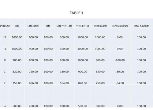
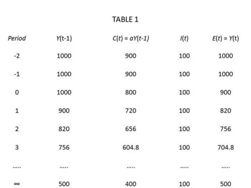
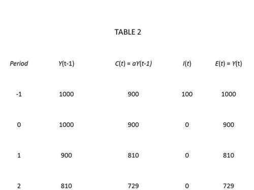
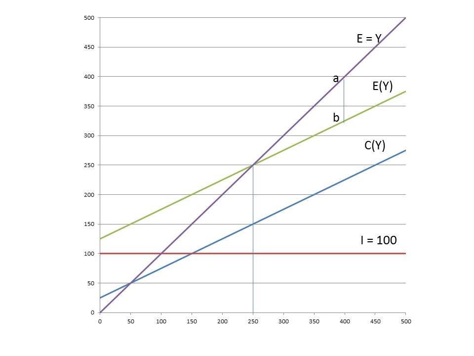
Keynes tried to show that the neoclassical theory could not possibly be right, inasmuch as, according to the theory, the equilibrium rate of interest is the rate that equilibrates the supply of with the demand for loanable funds. Keynes argued that because investment and savings are identically equal, savings and investment could not determine the rate of interest. But Keynes then turned right around and said that actually the equality of savings and investment determines the level of income. Well, if savings and investment are identically equal, so that the rate of interest can’t be determined by equilibrating the market for loanable funds, it is equally impossible for savings and investment to determine the level of income.

Keynes was unable to distinguish the necessary accounting identity of savings and investment from the contingent equality of savings and investment as an equilibrium condition. For savings and investment to determine the level of income, there must be some alternative definition of savings and investment that allows them to be unequal except at equilibrium. But if there are alternative definitions of savings and investment that allow those magnitudes to be unequal out of equilibrium — and there must be such alternative definitions if the equality of savings and investment determines the level of income — there is no reason why the equality of savings and investment could not be an equilibrium condition for the rate of interest. So Keynes’s attempt to refute the neoclassical theory of interest failed. That was Hawtrey’s criticism of Keynes’s use of the savings-investment accounting identity.

Pettis goes on to cite Keynes’s criticism of the Versailles Treaty in The Economic Consequences of the Peace as another example of Keynes’s adroit use of accounting identities to expose fallacious thinking.

A case in point is The Economic Consequences of the Peace, the heart of whose argument rests on one of those accounting identities that are both obvious and easily ignored. When Keynes wrote the book, several members of the Entente – dominated by England, France, and the United States – were determined to force Germany to make reparations payments that were extraordinarily high relative to the economy’s productive capacity. They also demanded, especially France, conditions that would protect them from Germany’s export prowess (including the expropriation of coal mines, trains, rails, and capital equipment) while they rebuilt their shattered manufacturing capacity and infrastructure.

The argument Keynes made in objecting to these policies demands was based on a very simple accounting identity, namely that the balance of payments for any country must balance, i.e. it must always add to zero. The various demands made by France, Belgium, England and the other countries that had been ravaged by war were mutually contradictory when expressed in balance of payments terms, and if this wasn’t obvious to the former belligerents, it should be once they were reminded of the identity that required outflows to be perfectly matched by inflows.

In principle, I have no problem with such a use of accounting identities. There’s nothing wrong with pointing out the logical inconsistency between wanting Germany to pay reparations and being unwilling to accept payment in anything but gold. Using an accounting identity in this way is akin to using the law of conservation of energy to point out that perpetual motion is impossible. However, essentially the same argument could be made using an equilibrium condition for the balance of payments instead of an identity. The difference is that the accounting identity tells you nothing about how the system evolves over time. For that you need a behavioral theory that explains how the system adjusts when the equilibrium conditions are not satisfied. Accounting identities and conservation laws don’t give you any information about how the system adjusts when it is out of equilibrium. So as Pettis goes on to elaborate on Keynes’s analysis of the reparations issue, one or more behavioral theories must be tacitly called upon to explain how the international system would adjust to a balance-of-payments disequilibrium.

If Germany had to make substantial reparation payments, Keynes explained, Germany’s capital account would tend towards a massive deficit. The accounting identity made clear that there were only three possible ways that together could resolve the capital account imbalance. First, Germany could draw down against its gold supply, liquidate its foreign assets, and sell domestic assets to foreigners, including art, real estate, and factories. The problem here was that Germany simply did not have anywhere near enough gold or transferable assets left after it had paid for the war, and it was hard to imagine any sustainable way of liquidating real estate. This option was always a non-starter.

Second, Germany could run massive current account surpluses to match the reparations payments. The obvious problem here, of course, was that this was unacceptable to the belligerents, especially France, because it meant that German manufacturing would displace their own, both at home and among their export clients. Finally, Germany could borrow every year an amount equal to its annual capital and current account deficits. For a few years during the heyday of the 1920s bubble, Germany was able to do just this, borrowing more than half of its reparation payments from the US markets, but much of this borrowing occurred because the great hyperinflation of the early 1920s had wiped out the country’s debt burden. But as German debt grew once again after the hyperinflation, so did the reluctance to continue to fund reparations payments. It should have been obvious anyway that American banks would never accept funding the full amount of the reparations bill.

What the Entente wanted, in other words, required an unrealistic resolution of the need to balance inflows and outflows. Keynes resorted to accounting identities not to generate a model of reparations, but rather to show that the existing model implicit in the negotiations was contradictory. The identity should have made it clear that because of assumptions about what Germany could and couldn’t do, the global economy in the 1920s was being built around a set of imbalances whose smooth resolution required a set of circumstances that were either logically inconsistent or unsustainable. For that reason they would necessarily be resolved in a very disruptive way, one that required out of arithmetical necessity a substantial number of sovereign defaults. Of course this is what happened.

Actually, if it had not been for the insane Bank of France and the misguided attempt by the Fed to burst the supposed stock-market bubble, the international system could have continued for a long time, perhaps indefinitely, with US banks lending enough to Germany to prevent default until rapid economic growth in the US and western Europe enabled the Germans to service their debt and persuaded the French to allow the Germans to do so via an export surplus. Instead, the insane Bank of France, with the unwitting cooperation of the clueless (following Benjamin Strong’s untimely demise) Federal Reserve precipitated a worldwide deflation that triggered that debt-deflationary downward spiral that we call the Great Depression.

Why Theories of National Income Based on Accounting Identities Are Nonsensical and Error-Ridden, Part IV

In my previous post, I tried to relate the discussion of accounting identities to the familiar circular-flow diagram with injections into and leakages out of the flows of income, expenditure and output. My hopes that framing the discussion in terms of injections and leakages, with investment viewed as an injection into, and savings as a withdrawal out of, the flows of income and expenditure would help clarify my position about accounting identities were disappointed, as defenders of those accounting identities were highly critical of the injections-leakages analogy, launching a barrage of criticism at my argument that the basic macroeconomic model of income determination should not be understood in terms of the income-expenditure or the investment-savings identities.

I think that criticism of the injections-leakages analogy was, for the most part, misplaced and a based on a misunderstanding of what I have been aiming to do, but much of the criticism was prompted by my incomplete or inadequate explanation of my reasoning. So, before continuing with my summary of Lipsey’s essay on the subject, on which this series is based, I need to address at least some of the points that have been made by my (and Lipsey’s) various critics. In the course of doing so, I believe it will be helpful if I offer a revised version of Lipsey’s Table 1, which I reproduced in part III of this series.

First, I am not saying that the standard accounting identities are wrong. Definitions are neither right nor wrong, but they may be useful or not useful depending on the context. In everyday conversation, we routinely ascribe one of many possible meanings to particular words used by selecting one of the many possible definitions as that which is most likely to make an entire sequence of words – a phrase, a clause, or a sentence – meaningful. Our choice of which definition to use is generally determined by the context in which the word appears. Choosing one definition over another doesn’t mean that others are not valid, just that the others would not work as well or at all in the context in which the word in question appears. Working with an inappropriate definition in a given context can lead, as we all know from personal experience, to confusion, misunderstanding and error. Defining savings and investment to be equal in every state of the world is certainly possible, and doing so is not invalid, but doing so is not necessarily useful in the context of formulating a macroeconomic theory of income determination.

There are two reasons why defining savings and investment to be identically equal in all states of the world is not useful in a macroeconomic theory of income. First, if we define savings and investment (or income and expenditure) to be identically equal, we can’t solve, either algebraically or graphically, the system of equations describing the model for a unique equilibrium. According to the model, aggregate expenditure is assumed to be a function of income, but if income and expenditure are identical, expenditure is simply identical to itself, so the system of equations described by the model collapses onto the 45-degree line representing the expenditure-income identity.

Second, even if we interpret the equality of income and expenditure as an ex ante equilibrium condition, while asserting that identity between income and expenditure must always hold ex post, the ex post definitional equality tells us nothing about the adjustment process that restores equilibrium when, owing to some parameter change that disturbs a pre-existing equilibrium, the ex ante equilibrium condition does not hold. For a dynamic adjustment path to take the model from one equilibrium to another via a sequence of discrete adjustments, the model must incorporate some lags. Without lags, the adjustment would be instantaneous, and the model would move from its old equilibrium to a new equilibrium in one fell swoop. But in the course of a sequence of partial adjustments, savings and investment will typically have to be defined by the model so that they are not equal, and this will be reflected in the implied course of savings and investment if the model is worked out period-by-period. Or if you were to observe the Phillips machine (a hydraulic macroeconomic model built by A. W. Phillips of Phillips Curve fame) in action, you could actually see that the savings and investment flows were of unequal magnitudes as machine responded to a change in the settings and moved from one hydraulic equilibrium to another.

It is a common mistake, and the primary object of Richard Lipsey’s scorn in his essay, to attribute causal significance to the savings-investment identity, as if it were the force of the identity itself that guided the dynamic adjustment, when, in reality, the identity, which can always be recovered if one does all the necessary accounting and classifies all the transactions according to the accounting conventions, is irrelevant to the adjustment path. Doing the accounting does not explain how the model moves from the old to a new equilibrium; it just assures us that nothing has been omitted from a final description of what has happened. Rather, the causal mechanism driving the adjustment process can be described using the intuitive idea that income changes because there are injections (in the form of investment) into the income and expenditure flows and leakages (in the form of savings) out of those flows, and when the injections and leakages are unequal in magnitude, the discrepancy between the injections and the leakages causes a corresponding change in the income and expenditure flows.

One commenter pointed out that, even in the numerical example (taken from Lipsey’s essay) that I gave in my earlier post, the sequence of adjustments preserved the definitional equality between savings and investment and income and expenditure, even though the verbal explanation of the adjustment process showed that the equality of savings and investment required a rather forced interpretation of the meaning of savings: the difference between the cash balance expected at the end of a period and the actual cash balance at the end of the period. This peculiar interpretation of savings and its equality with investment reflected the way that Lipsey chose to introduce a lag between expenditure and income into the model: by assuming that income was disbursed by businesses to households at the end of the period in which households provide services to businesses. The income received at the end of one period is then used to finance consumption expenditures and savings in the following period.

I should have pointed out that if one made the trivial adjustment in the expenditure-income lag, so that incomes earned in one period are not at the end of the current period, but at the beginning of the following period, then income and expenditure and savings and investment would not remain equal over the course of the adjustment from the old to the new equilibrium. The sequence of adjustments under the alternative assumption is shown in Table 1 below.

Of course, if we assume that there is a one-period lag between expenditure and income, one could define something called total savings, which would be household savings plus business savings, where business savings is defined as the difference between cash held by businesses at the end of the current period and cash held by businesses at the end of the previous period. And total savings is identically equal to investment. However, it is important to bear in mind that from the point of view of the simple income-expenditure model, the relevant causal variable in determining equilibrium is not total savings, but household savings.

Why do I say that household savings, not business savings, is the relevant causal factor in determining equilibrium income in the simple income-expenditure model? The reason should be obvious: the solution for equilibrium in the simple income-expenditure model is Y = A/(1 – MPC), where A represents the autonomous component of consumption plus planned investment by business firms and MPC is the marginal propensity to consume by households, so that (1 – MPC) is the marginal propensity to save (MPS) . . . by households!

In this setup, business savings is a pure residual adjusting to make up the difference between household savings and investment. When household savings exceeds investment, businesses accumulate their holdings of cash, and when investment is greater than household saving, businesses reduce their accumulate cash. The operation of the banking system might be relevant at this point, but that analysis would take this discussion to a whole new level, which I am not going to get started on at this point.

I will close at this point by just saying that I think that I have provided an answer to the following comment on my previous post asking what is gained by introducing an alternative set of definitions of saving and investment under which savings and investment are equal only in equilibrium, but not otherwise:

But let’s just say you have a system of accounts where definitions are different and saving is different from investment. I can do a mathematical transformation to a new set of variables in which standard identities hold. What is the point of writing so much? Absolutely nothing.

The point of course is that by defining savings and investment so that they are equal only in equilibrium, we now have a system of two linear equations in two unknowns that can be solved for a unique solution, something that cannot be done if savings and investment are identically equal. Second, when we have defined savings and investment so that they can be unequal, but define their equality to be a condition of equilibrium, we can write the following dynamic relationships characterizing the system:

dY/dt = 0 <=> I = S

dY/dt > 0 <=> I > S

dY/dt < 0 <=> I < S

where I and S are defined under the behavioral assumptions in this example as actual investment by businesses and saving by households. The precise definition of I and S would depend, in each particular case, on the specific behavioral assumptions about the underlying lag structure of the model for that particular case. The definitional equality of total savings and investment has no causal significance, but simply reflects the fact that total savings is defined in such a way that it must equal investment.

The definitional equality of savings and investment, as Scott Sumner has observed, is exactly analogous to the quantity identity MV ≡ PY, when V is treated not as the reciprocal of the amount of money demanded as a fraction of income — which is to say as a measurable magnitude understood to be a function of specifiable independent variables — but simply as a residual whose value, by definition, must always be identically equal to PY/M. The quantity identity, lacking being consistent with all possible states of the world, because V is defined not as an independent variable, but as a mere residual. The quantity identity is therefore of no use in describing the dynamic process of adjustment to a change in the quantity of money or what in telling us what are the causes of such a process.

UPDATE (3/29/15): In writing a response to Jamie’s comment, I realized that in the third paragraph after the table above, I misstated the relationship between business savings and the difference between investment and household savings. I have made the correction, and apologize for not being more careful.

Of Bathtubs, Drains, and Faucets

I was planning to write another installment in my series of posts on the savings-investment identity in which I have been working through and summarizing Richard Lipsey’s essay “The Foundations of the Theory of National Income.” Perhaps I will get to my next installment later this week. If not, then I hope to do so early next week. But it occurred to me that the best way to explain why saving is not identical to investment is by framing the discussion in terms of the familiar circular-flow schematic model of income and expenditure. The accompanying diagram is a typical representation of the circular-flow model, with a government sector (government spending and taxes) and a foreign sector (exports and imports) included in addition to just circular_flow_modelinvestment and saving.

As indicated by the arrows in the diagram, investment, government spending, and exports are added to the circular flow while savings, taxes and imports are withdrawn from the circular. In the conventional terminology, investment, government spending and exports are injections, and savings, taxes and imports are leakages. And, of course, a basic property of the model is that injections and leakages are equal. It is only in the simplest model, with no government and with no foreign sector, so that there is just one injection (investment) and one leakage (saving), in which the familiar equality between investment and savings holds.

So the question that I want to ask now is simply this: is the equality in the simple one-sector model between injections (investment) and leakages (savings) an equality that may or may not be true, or is it an identity that must necessarily be satisfied in all places and at all times?

Well, rather than try to argue this through in terms of abstract economic or accounting reasoning, let’s think about it in terms of a simple physical analogy, one that we could actually demonstrate for ourselves in our own homes. So think of a bathtub with some water in it. Depending on the size of the bathtub and the amount of water in the bathtub, the water will reach some uniform height in the bathtub. Let’s call that uniform water level an equilibrium. It’s an equilibrium, because if that’s all the water there is in the bathtub, and we don’t let any water out of the bathtub, and, for purposes of our little thought experiment, we ignore any evaporation, that water level will persist indefinitely, with no tendency to change. No water in, no water out, and you have a constant water level. In other words, with no injections and no leakages, the water level of the bathtub is stable; it does not change. The water level is in equilibrium.

But if you turn on the faucet and water starts to flow into the bathtub, the water level will start to rise. As long as water is being injected into the bathtub, the water level will keep rising, and the water level will not be in equilibrium. However, if you unplug the drain to the bathtub, water will start flowing out of the bathtub. What happens to the water level? That depends on whether water is leaking out of the bathtub through the drain faster than water is being injected into the bath tub through the faucet. If injections are greater than leakages, the water level will rise, and if leakages are greater than injections, the water level will fall. And if, by chance or design, injections are exactly equal to leakages, then the water level will be stable and back in equilibrium. Thus, the condition for a stable water level is that injections be exactly equal to leakages. When injections into, and leakages from, the bathtub are equal, the water level of the bathtub is in equilibrium. When injections are greater than leakages, the water level rises, and when leakages are greater than injections the water level falls.

I think all that is pretty elementary, and I am guessing that if you look in any textbook treatment of injections and leakages in the circular flow of income, you will find a similar story about the effect of a difference between injections and leakages on the level of income. (Check out the Wikipedia article on the circular flow of income, especially the section on equilibrium.)

So, if you believe that investment and savings are identically equal, please tell me whether you also believe that injections and leakages are identically equal. And if you do believe that injections and leakages are identically equal, please explain to me what the difference is between the circular-flow-of-income model with injections and leakages identically equal in equilibrium or out of equilibrium and the bathtub model in which the water level can change only insofar as injections and leakages are not equal.

Why Theories of National Income Based on Accounting Identities Are Nonsensical and Error-Ridden, Part III

In my previous post, I argued that an accounting identity, which tells us that two expressions are defined to be the same, must hold in every state of the world, and therefore could not be disproved by any conceivable observation. So if I define savings and investment (or income and expenditure) to be the same thing, I am simply restricting my semantic description of the world, I am not restricting in any way the set of observable states of the world that conform to my semantic convention. An accounting identity therefore has no empirical content, which means that the accounting identity between savings and investment cannot explain the process by which a macroeconomic model adjusts to a parametric change in the model, traversing from a pre-existing equilibrium with savings and investment being equal to a new equilibrium with savings and investment equal.

In his paper, “The Foundations of the Theory of National Income,” which I am attempting to summarize and explain in this series of posts, R. G. Lipsey provides a numerical example of such an adjustment path. And it will be instructive to follow that path in some detail. The key point about this model is the assumption that households decide how much to save and consume in the current period based on the disposable income received in the previous period. The assumption that all receipts of the business firms are paid out to owners and providers of factor services at the end of each period is a behavioral assumption (not an accounting identity) that rules out any change in the retained earnings held by firms. If firms were accumulating financial assets, then their payments to households would not match their receipts. The following simple model reflects a one-period lag (known as a Robertsonian lag) between household earnings and household consumption.

C(t) = aY(t-1) (behavioral assumption)

I(t) = I* (behavioral assumption)

E(t) ≡ C(t) + I(t) (accounting identity)

Y(t) ≡ C(t) + S(t) (accounting identity)

Y(t) = E(t) (behavioral assumption)

Y(t-1) = Y(t) (equilibrium condition)

Assume that the economy starts off with a = .9 and I(t) = 100. The system is easily solved for E = Y = 1000, with C = 900 and I = 100. Savings, which is the difference between Y and C, is 100, just equal to I. The definition of saving will have to be fleshed out further below. Now assume that there is a parametric change in a (the marginal propensity to consume) to .8 from .9. This change causes equilibrium income to fall from 1000 to 500. By assumption, investment is constant, so that in the new equilibrium saving remains equal to 100. The change in income is reflected in a drop in consumption from 900 to 400. But given the one-period lag between earnings and expenditure, we can follow how the system changes over time, moving closer and closer to the new equilibrium in each successive period, as shown in the following table.

Consider the following questions.

First, in the course of this period-by-period adjustment, will there be any unplanned investment?

Second, in this example, the parametric change — an increase in the propensity of households to save — may be described as an increase in planned savings by households. Planned investment is unchanged. With planned savings greater than planned investment, will the household plans to increase savings be frustrated (implying positive or negative unplanned savings) as alleged in proposition 3 in the list of erroneous propositions provided earlier in the first installment in this series (see appendix below).

The answer to the first question is: not necessarily. There is nothing to prevent us from assuming that all firms correctly anticipate the reduction in consumer demand, so that production falls along with consumption with no change in inventories. It is not necessary to assume that firms can foresee the future; it could be that all consumption is in the form of services, or that production is undertaken only in response to consumer orders. With inventories unchanged, there is no unplanned investment.

The answer to the second question is that it depends on what is meant by unplanned savings. Unplanned savings could mean that households wind up saving an amount other than the amount that they had intended to save at the beginning of the period; households intended to save 200 at the beginning of period 0, but because their income turned out to be only 900, instead of 1000, in period 0, household savings, under the accounting identity, is only 100 instead of 200. However, households intended to consume 800 in period 0, and that is the amount that they actually consumed. The only sense in which households did not execute their intended plans is that household income in period 0 was less than households had expected. Lipsey calls this a distinction between plans in the point sense, and plans in the schedule sense. In this scenario, while plans in the schedule sense are carried out, plans in the point sense are not, because households do not end up at the point on their consumption functions that they had expected to be on.

So the equilibrium condition above that income does not change from one period to the next can be restated as follows: the system is in equilibrium when planned savings equals realized savings. Planned savings is the unconsumed portion of households’ expected income, which is the income households earned in the previous period. The definition embodies a specific behavioral hypothesis about how households formulate their expectations of income in the future.

S_p_(t) ≡ Y(t-1) – C(t).

Realized savings is the unconsumed portion of households’ actual income in the current period. It can be written as

S_r_(t) ≡ Y(t) – C(t).

Or restated differently yet again, the equilibrium condition is that actual disposable income in period t equals expected disposable income in period t.

Let’s flesh out the behavioral assumptions behind this model in a bit more detail. Business firms disburse income to households (owners and providers of factor services) at the end of each period. Households decide how much to save and consume in the upcoming period after receiving their incomes from firms at the close of the previous period. Savings are in the form of bond purchases made at the start of the period. Based on the consumption and savings plans formulated by households at the start of the new period, firms decide how much output to produce and how much labor to hire to produce that output, firms immediately notifying households how many hours they will work in the upcoming period. However, households are committed to the consumption plans already made at the beginning of the period, so they must execute those plans even if the incomes earned during the period are less than anticipated.

In our example, by choosing to increase their savings to 200 through bond purchases at the beginning of the upcoming period, while reducing consumption from 900 to 800, households cause business firms to reduce output from 1000 to 900 (investment being unchanged), and to reduce employment (measured in terms of total hours worked) by 11.1%. After buying bonds equal to 200, households have 800 left in cash, with which they finance their purchases for the rest of the month. So it is not obvious that households were unable to execute any of their plans  during the period. However, at the end of the period, households receive only 900 in income from business firms, so although households did buy bonds equal to 200 at the start of the period, they carry over only 900 in cash into the next period, not 1000 as expected. Thus, realized savings are only 100 instead of 200, because household cash holding at the endo f the period turned out to be 100 less than expected. Nevertheless, it is difficult to identify any plan to save that was frustrated, inasmuch as households did purchase bonds equal to 200 at the beginning of the period, and did reduce consumption as planned. As Lipsey puts it:

[W]hether or not the actual real plans laid by households are frustrated depends on what plans households lay, i.e., it depends on our behaviour assumption, not on our definitions. If we assume that households make point plans about their bonds, and schedules plans about their transactions and precautionary balances, then no frustration of plans occurs.

If the statement quoted in (3) [see appendix below] is meant to have empirical content, it depends on a very specific hypothesis about households’ savings plans. These plans must be made in the point and not in the schedule sense, and the plans must include not only additions to the stock of income-earning assets, but also point-plans concerning transactions balances even though the household does not now know what level of transactions the balances will be required to facilitate. . . .

[W]e are now in a position to see what is wrong with statement (2), that actual savings must always equal actual investment, and statement (5), which draws the analogy with demand and supply analysis. Consider statement (2) first.

In the General Theory, Keynes stressed the fact that savings and investment decisions are made by different groups and that there is thus, no reason why planned investment should equal planned savings. [It has been argued] that, although plans can differ, actual realised saving must always be equal to actual realised investment, and, therefore, when planned savings does not equal planned investment, either the plans of savers, or of investors, must be frustrated. Of course, it is quite possible to define savings and investment so that they are the same thing, but it is a basic error to equate the magnitude so defined with the magnitude about which savers actually lay plans. Since ex post S and I as defined bear no relation to the magnitudes about which savers actually make plans, we can deduce nothing about what happens when ex ante S is not equal to ex ante I from the fact that we chose to use the terms ex post S and ex post I to refer to a single, and different, magnitude. The basic error arises from the assumption that households and firms make plans about the same magnitude when they are planning their savings and investment. The traditional theory defines investment as goods produced and not sold to households (= capital goods plus changes in inventories). According to our theory of the behaviour of firms, this is what firms do lay plans about: they plan to add so many capital goods and so many inventories to their existing holdings. The theory then says I ≡ S, and , thus, builds in the implicit assumption that households lay plans about the same magnitude. But according to the standard theory of household behaviour, they do not do so! Households, not subject to money illusion, are assumed to wish to lay aside a certain quantity of real purchasing power which is either used to increase the holdings of cash or used to purchase bonds. There is nothing in the standard theory of household behaviour that leads us to hypothesise that households care whether or not there exists – produced but unconsumed – a physical stock of goods which is the counterpart of the money they have laid aside. Indeed why should they? All they are assumed to care about is the potential real purchasing power of their savings, and this depends only on the amount of money saved, the present price level, and the expected future price level.

This is one of the keys to the whole present confusion: households lay plans about a magnitude that is different from the one that firms lay plans about. Firms plan to have produced and unconsumed a certain quantity of goods, while households plan to leave unspent a certain quantity of purchasing power. This means that it is quite possible for planned investment to differ from planned savings and to have both sets of plans fulfilled so that actual, realized investment differs from actual realized savings. [footnote: Now, of course, we mean by realised S and I the realised magnitudes about which firms and households are actually laying plans. This, of course, does not interfere with the statistician saying that realised savings is identical with realised investment since he refers to a different magnitude when he speaks of realised savings.]

Now consider another variation of the numerical example in Table 1. Instead of a change in the propensity to consume in period 0, assume instead that planned investment drops from 100 to 0. Starting with period -1, Table 2 displays the same initial equilibrium as in Table 1. Because we make a behavioral hypothesis that inventories do not change, planned and realized investment must be zero in period 0 and in all subsequent periods.

According to the national-income identities, savings must equal zero because investment is zero. But what is the actual behavior that corresponds to zero saving? In period 0, households carried over 1000 in cash from period -1. From that 1000, they used 100 to buy bonds and spent the remainder of their disposable incomes on consumption goods. So households planned to save 100 and consume 900, and it appears that they succeeded in executing their plans. But according to the national-income identities, they failed to execute their plan to save 100, and saved only 0, presumably because there were unintended savings of -100 that cancelled out the planned (and executed) savings of 100. So it appears that we have come up against something of a paradox. Here is Lipsey’s solution of the paradox.

[A]ny definitions are possible if consistently used, but this use of the word “unintended” has nothing to do with intended and unintended behaviour. To preserve the identity we must say that the plans of households were frustrated because a real counterpart of the saving they successfully made was not produced. We may say this if we wish, but the danger is that we will think we have said something about the world, and about the actual experiences of households. Indeed, a perusal of established textbooks shows that this confusion has occurred over and over again.

Thus, we conclude that, when we define investment as production not consumed, and savings as income [not consumed] . . . there is no reason why actual savings should not differ from actual investment.

Finally, what about the analogy between savings and investment in macro analysis and demand and supply in micro analysis as in erroneous statement (4) (see appendix)? If we write demand for some good as a function of the price of the good

D = D(p),

and write the supply of some good as a function of the price of the good

S = S(p),

then our equilibrium condition is simply D = S, where D represents desired purchases of the good, and S represents desired sales of the good. Because the act of selling logically entails the activity of purchasing, a purchase and a sale are merely different names for the same thing. So the plans of demanders to buy and the plans of suppliers to sell are plans about the same thing. The plans of demanders to buy and the plans of suppliers to sell cannot be fulfilled simultaneously unless there is an equilibrium in which demand equals supply. The difference between the microeconomic equilibrium in which demand equals supply and the macroeconomic equilibrium in which savings equals investment is that suppliers and demanders in a market are making plans about the same magnitude: sales (aka purchases) of a good. However,

in the national income case the two sets of real plans (savers’ and investors’) are laid about two different magnitudes. Thus the analogy often draw between the two theories in respect of plans and realized quantities is an incorrect one.

Appendix: List of Erroneous Propositions

1 The equilibrium of the basic Keynesian model is given by the intersection of the aggregate demand (i.e., expenditure) function and the 45-degree line representing the accounting identity EY.

2 Although people may try to save different amounts from what people try to invest, savings can’t be different from investment; realized (ex post) savings necessarily always equals realized (ex post) investment.

3 Out of equilibrium, planned savings do not equal planned investment, so it follows from (2) that someone’s plans are being disappointed, and there must be either unplanned savings or dissavings, or unplanned investment or disinvestment

4 The simultaneous fulfilment of the plans of savers and investors occurs only when income is at its equilibrium level just as the plans of buyers and sellers can be simultaneously fulfilled only at the equilibrium price.

5 Whenever savers (households) plan to save an amount different from what investors (business firms) plan to invest, a mechanism operates to ensure that realized savings remain equal to realized investment, despite the attempts of savers and investors to make it otherwise. Indeed, this mechanism is what causes dynamic change in the circular flow of income and expenditure.

6 Since the real world, unlike the simple textbook model, contains a very complex set of interactions, it is not easy to see how savings stay equal to investment even in the worst disequilibrium and the most rapid change.

7 The dynamic behavior of the Keynesian circular flow model in which disequilibrium implies unintended investment or disinvestment can be shown by moving upwards or downwards along the gap between the expenditure function and the 45-degree line in the basic Keynesian model.

Why Theories of National Income Based on Accounting Identities Are Nonsensical and Error-Ridden, Part II

In this installment of my series on Richard Lipsey’s essay “The Foundations of the Theory of National Income,” I am going to focus on a single issue: what inferences about reality are deducible from a definition about the meaning of the terms used in a scientific theory? In my first installment I listed seven common statements about the basic Keynesian income-expenditure model that are found in most textbooks. The first concerned the confusion between the equality of investment and saving (or between income and expenditure) as an equilibrium condition and a definitional identity. Interpreting the equality of savings and investment as an identity essentially means collapsing the entire model onto the 45-degree line and arbitrarily choosing some point on the 45-degree line as the solution of the model.

That nonsensical interpretation of the simple Keynesian cross is obviously unsatisfactory, so, in an effort to save both the definitional identity of savings and investment and the equality of investment and savings as an equilibrium condition, the textbooks have introduced a distinction between ex ante and ex post in which savings and investment are defined to be identically equal ex post, but planned (ex ante) savings may differ from planned (ex ante) investment, their equality being the condition for equilibrium.

Now, to be fair, it is perfectly legitimate to define an equilibrium in terms of plan consistency, and to say that the inconsistency of the plans occasions a process of readjustment in the plans, and that it is the readjustment in the plans which leads to a new equilibrium. The problem with the textbook treatment is that it draws factual inferences about the adjustment process to a disequilibrium in which planned saving is not equal to planned investment from the definitional identity between ex post savings and ex post investment. In particular, the typical textbook treatment infers that in a disequilibrium with planned savings not equal to planned investment, the adjustment process is characterized by unplanned positive or negative investment (inventory accumulation or decumulation) corresponding to the gap between planned savings and planned investment. Identifying a gap between planned saving and planned investment with unplanned inventory accumulation or decumulation, as textbook treatments of the income expenditure model typically do, is logically unfounded.

Again, I want to be careful, I am not saying that unplanned inventory accumulation or decumulation could not occur in response to a difference gap between planned savings and planned investment, or even that such unplanned inventory accumulation or decumulation is unlikely to occur. What I am saying is that the definitional identity between ex post savings and ex post investment does not imply that such inventory accumulation or decumulation takes place and certainly not that the amount by which inventories change is necessarily equal to the gap between planned savings and planned investment.

Richard Lipsey made the key point in his comment on my previous post:

The main issue in this whole discussion is, I think, can we use a definitional identity to rule out an imaginable state of the universe. The answer is “No”, which is why Keynes was wrong. The definitional identity of S ≡ I tells us nothing about what will happen if agents wish to save a different amount from what agents wish to invest.

Here is how Lipsey put it in his 1972 essay:

The error in this interpretation lies in the belief that the identity EY can tell us what can and cannot happen in the world. If it were possible that a definitional identity could rule out certain imaginable events, then such a definitional identity would be an informative statement having empirical content! If it is a genuine definitional identity (which follows from our use of words and is compatible with all states of the universe) then it is only telling us that we are using E and Y to refer to the same thing, and this statement no more allows us to place restrictions on what happens in the world than does the statement that we are not using E and Y to refer to the same thing.

Lipsey illustrated the problem using the simple Keynesian cross diagram. To make the discussion a bit easier to follow, I am going to refer to my own slightly altered version (using a specific numerical example) of the familiar diagram. Setting investment (I) equal to 100 and assuming the following consumption function

C = 25 + .5Y

We can easily solve for an equilibrium income of 250 corresponding to the intersection of the expenditure function with the 45-degree line.

lipsey_45_degreeWhat happens if we posit that the system is at a disequilibrium point, say Y = 400. The usual interpretation is that at Y = 400, planned (ex ante) investment is less than savings and planned (ex ante) expenditure is less than income. Because, actual (ex post) investment is identically equal to savings and because actual (ex post) expenditure is identically equal to income, unplanned investment must occur to guarantee that the investment-savings identity is satisfied. The amount of unplanned investment is shown on the graph as the vertical distance between the expenditure function (E(Y)) at Y = 400 and the 45-degree line at Y = 400. This distance is shown in my diagram as the vertical distance between the points a and b on the diagram, and it is easy to check that the distance corresponds to a value of 75.

So the basic textbook interpretation of the Keynesian cross is using the savings-investment identity to derive a proposition about the behavior of the economy in disequilibrium. It is saying that an economy in disequilibrium with planned investment less than planned savings adjusts to the disequilibrium through unplanned inventory accumulation (unplanned investment) that exactly matches the difference between planned saving and planned investment. But it is logically impossible for a verbal identity (between savings and investment) — an identity that can never be violated in any actual state of the world — to give us any information about what actually happens in the world, because whatever happens in the world, the identity will always be satisfied.

Recall erroneous propositions 2, 3 and 4, listed in part I of this series:

2 Although people may try to save different amounts from what people try to invest, savings can’t be different from investment; realized (ex post) savings necessarily always equals realized (ex post) investment.

3 Out of equilibrium, planned savings do not equal planned investment, so it follows from (2) that someone’s plans are being disappointed, and there must be either unplanned savings or dissavings, or unplanned investment or disinvestment

4 The simultaneous fulfilment of the plans of savers and investors occurs only when income is at its equilibrium level just as the plans of buyers and sellers can be simultaneously fulfilled only at the equilibrium price.

If realized (ex post) savings necessarily always equals realized (ex post) investment, that equality is the result of how we have chosen to define those terms, not because of people actually are behaving, e.g., by unwillingly accumulating inventories or failing to save as much as they had intended to. However people behave, the identity between savings and investment will be satisfied. And whether savers and investors are able to fulfill their plans or are unable to do so cannot possibly be inferred from a definition that says that savings and investment mean the same thing.

In several of his comments on my recent posts, Scott Sumner has cited the professional consensus that savings and investment are defined to be equal. I am not so sure that there is really a consensus on that point, because I don’t think that most economists have thought carefully about what the identity actually means. But even if there is a consensus that savings is identical to investment, no empirical implication follows from that definition. But typical textbook expositions, and I think even Scott himself when he is not being careful, do use the savings-investment identity to make inferences about what actually happens in the real world.

In the next installment, I will go through a numerical example that shows, based on a simple lagged adjustment between consumption and income (household consumption in this period being a function of income in the previous period), that planned savings and planned investment can be realized and unequal in the transition from one equilibrium to another.

PS I apologize for having been unable to respond to a number of comments to previous posts. I will try to respond in the next day or two.

Imagination and Identity

Before continuing my summary of the key points of Richard Lipsey’s important paper, “The Foundations of the Theory of National Income,” I want to clear up a point that the deliberately provocative title may have obscured. The accounting identities that I am singling out for criticism are the identities between income and expenditure (and output) and between savings and investment. It is true that, as Scott Sumner points out in a comment on my previous post, every theory has to define its terms in some way or another, so there is no point in asserting that a definition is wrong. Scott believes that I am a saying that it is wrong to define investment and savings as the same thing, but I am not saying that. I am saying that, in the context of the basic income-expenditure theory of national income, it makes the theory incoherent, so that there is a mismatch between the definition and the theory.

It is also true that sometimes identities follow directly from basic definitions. Such identities are like conservation laws in physics. For example, purchases must equal sales, because purchasing and selling are reciprocal activities; to assert that purchases are, or could be, unequal to sales would be self-contradictory. Keynes, when ridiculed by Hawtrey for asserting that a) savings and investment are equal by definition, and b) that the equality of savings and investment is achieved by variations in income, responded by comparing the equality of savings and investment to the equality of purchases and sales. Purchases are necessarily equal to sales, but prices adjust to achieve equality between desired purchases and desired sales.

The problem with Keynes’s response to Hawtrey is that to assert that purchases are unequal to sales is to misconstrue in a really fundamental way the meaning of the terms “purchase” and “sales.” But when it comes to national-income accounting, the identity of “investment” and “savings” does not follow immediately from the meaning of those terms. It must be derived from the meaning of two other terms: income and expenditure. So the question becomes whether the act of spending (i.e., expenditure) necessarily entails an immediate and corresponding accrual of income, in the same way that the act of purchasing necessarily entails the act of selling. To assert that expenditure and income are identical is then to assert that any expenditure necessarily and simultaneously entails a corresponding accrual of income.

Before pursuing this line of thought further, let’s just pause for a moment to recall the context for this discussion. We are talking about a fairly primitive model of an economy in which there are households that are units of consumption and providers of factor services. Households purchase consumption goods and provide factor services to business firms. Business firms are units of production that combine factor services provided by households with raw materials purchased from other business firms, and new or existing capital goods produced now or previously by other business firms, to produce raw materials, consumption goods, and capital goods. Raw materials and capital goods are sold to other business firms and consumption goods are sold to households. Business firms are owned by households, so profits earned by business firms are remitted, along with payments for factor services, to households. But although the flow of payments from households to business firms corresponds to a flow of payments from business firms to households, the two flows, which can be measured separately, are, at not identical, or at least not obviously so. When I bought a tall Starbucks coffee just now at a Barnes & Noble cafe, my purchase of $1.98 was exactly and necessarily matched by a sale by Barnes & Noble to the guy who writes for the Uneasy Money blog. But expenditure of $1.98 by the Uneasy Money blogger to Barnes & Noble did not trigger an immediate and corresponding flow of $1.98 to households from Barnes & Noble.

Now I grant that it is possible for income so to be defined that every act of expenditure involves a corresponding accrual of income to providers of factor services to the firm, and of profit to owners of the firm. But expenditure entails simultaneous accrual of income only by virtue of an imputation of income to providers of factor services and of profit to owners of firms. Mere imputation does not and cannot constitute an actual flow of payments by firms to households. The identity between purchases and sales is entailed by the definition of “purchase” and “sales,’ but the supposed identity between expenditure and income is entailed by nothing but an act of imagination. I am not criticizing imagination, which may often provide us with an excellent grasp of reality. But imagination, no matter how well attuned to reality, does not and cannot establish identity.

Why Theories of National Income Based on Accounting Identities Are Nonsensical and Error-Ridden, Part I

I have had occasion to make many references in the past to Richard Lipsey’s wonderful article “The Foundations of the Theory of National Income” which was included in the volume Essays in Honour of Lord Robbins. When some 40 years ago, while a grad student at UCLA, I luckily came upon Lipsey’s essay, it was a revelation to me, because it contradicted what I had been taught as an undergrad about the distinctions between planned (ex ante) investment and savings, and realized (ex post) investment and savings. Supposedly, planned investment and planned savings are equal only in equilibrium, but realized investment and savings are always equal. Lipsey explained why the ex ante/ex post distinction is both incorrect and misleading. In this post I want to begin to summarize some of the important points that Lipsey made in his essay.

Lipsey starts with a list of seven erroneous propositions commonly found in introductory and intermediate textbooks. Here they are (copied almost verbatim), grouped under three headings:

I The Static Model in Equilibrium

1 The equilibrium of the basic Keynesian model is given by the intersection of the aggregate demand (i.e., expenditure) function and the 45-degree line representing the accounting identity EY.

II The Static Model in Disequilibrium

2 Although people may try to save different amounts from what people try to invest, savings can’t be different from investment; realized (ex post) savings necessarily always equals realized (ex post) investment.

3 Out of equilibrium, planned savings do not equal planned investment, so it follows from (2) that someone’s plans are being disappointed, and there must be either unplanned savings or dissavings, or unplanned investment or disinvestment

4 The simultaneous fulfilment of the plans of savers and investors occurs only when income is at its equilibrium level just as the plans of buyers and sellers can be simultaneously fulfilled only at the equilibrium price.

III The Dynamic Behavior of the Model

5 Whenever savers (households) plan to save an amount different from what investors (business firms) plan to invest, a mechanism operates to ensure that realized savings remain equal to realized investment, despite the attempts of savers and investors to make it otherwise. Indeed, this mechanism is what causes dynamic change in the circular flow of income and expenditure.

6 Since the real world, unlike the simple textbook model, contains a very complex set of interactions, it is not easy to see how savings stay equal to investment even in the worst disequilibrium and the most rapid change.

7 The dynamic behavior of the Keynesian circular flow model in which disequilibrium implies unintended investment or disinvestment can be shown by moving upwards or downwards along the gap between the expenditure function and the 45-degree line in the basic Keynesian model.

Although some or all of these propositions are found in most standard textbook treatments of national income theory, every one of them is wrong.

Let’s look at proposition 1. It says that the equilibrium level of income and expenditure is determined algebraically by the following two relations: the expenditure (or aggregate demand) function:

E = E(Y) + A

and the expenditure-income accounting identity

E ≡ Y.

An accounting identity provides no independent information about the real world, because there is no possible state of the world in which the accounting identity does not hold. It therefore adds no new information not contained in the expenditure function. So the equilibrium level of income and expenditure must be determined on the basis of only the expenditure function. But if the expenditure function remains as is, it cannot be solved, because there are two unknowns and only one equation. To solve the equation we have to make a substitution based on the accounting identity E ≡ Y. Using that substitution, we can rewrite the expenditure function this way.

E = E(E) + A

If the expenditure function is linear, we can write it as follows:

E = bE + A,

which leads to the following solution:

E = A/(1 – b).

That solution tells us that expenditure is a particular number, but it is not a functional relationship between two variables representing a theory, however naïve, of household behavior; it simply asserts that E takes on a particular value.

Thus treating the equality of investment and savings as an identity turns the simply Keynesian theory into a nonsense theory.

The point could be restated slightly differently. If we treat the equality of investment and savings as an identity, then if we follow the usual convention and label the vertical axis as E, it is a matter of indifference whether we label the horizontal axis Y or E, because Y and E are not distinct, they are identical. However we choose to label the horizontal axis, the solution of the model must occur along the 45-degree line representing either E = Y or E = E, which are equivalent. Because, the equality between E and itself or between E and Y is necessarily satisfied at any value of E, we can arbitrarily choose whatever value of E we want, and we will have a solution.

So the only reasonable way to interpret the equality between investment and saving, so that you can derive a solution to the simple Keynesian model is to treat E and Y as distinct variables that may differ, but will always be equal when the economy is in equilibrium.

So the only coherent theory of income is

E = E(Y) + A

and, an equilibrium condition

E = Y.

E and Y do not represent the same thing, so it makes sense to state a theory of how E varies in relation to Y, and to find a solution to the model corresponding to an equilibrium in which E and Y are equal, though they are distinct and not necessarily equal.

But the limitation of this model is that it provides us with no information about how the model behaves when it is not in equilibrium, not being in equilibrium meaning that E and Y are not the equal. Note, however, that if we restrict ourselves to the model in equilibrium, it is legitimate to write EY, because the equality of E and Y is what defines equilibrium. But all the erroneous statements 2 through 7 listed above all refer to how the model.

The nonsensical implications of constructing a model of income in which expenditure is treated as a function of income while income and expenditure are defined to be identical has led to the widespread adoption of a distinction between planned (ex ante) investment and savings and realized (ex post) investment and savings. Using the ex ante/ex post distinction, textbooks usually say that in equilibrium planned investment equals planned savings, while in disequilibrium not all investment and savings plans are realized. The reasoning being that is that if planned saving exceeds planned investment, the necessity for realized savings to equal realized investment requires that there be unintended investment or unintended dissaving. In other words, the definitional identity between expenditure and income is being used to tell us whether investment plans are being executed as planned or being frustrated in the real world.

Question: How is it possible that an identity true by definition in all states of the world can have any empirical implications?

Answer: It’s not.

In my next installment in this series, I will go through Lipsey’s example showing how planned and realized saving can indeed exceed planned and realized investment over the disequilibrium adjustment induced by a reduction in planned investment relative to a pre-existing equilibrium.

UPDATE (2/21/2015]: In the second sentence of the paragraph beginning with the words “An accounting Identity provides,” I wrote: “It therefore adds information not contained in the expenditure function,” which, of course, is the exact opposite of what I meant to say. I should have written: “It therefore adds NO NEW information not contained in the expenditure function.” I have now inserted those two words into the text. Thanks to Richard Lipsey for catching that unfortunate mistake.


About Me

David Glasner
Washington, DC

I am an economist in the Washington DC area. My research and writing has been mostly on monetary economics and policy and the history of economics. In my book Free Banking and Monetary Reform, I argued for a non-Monetarist non-Keynesian approach to monetary policy, based on a theory of a competitive supply of money. Over the years, I have become increasingly impressed by the similarities between my approach and that of R. G. Hawtrey and hope to bring Hawtrey’s unduly neglected contributions to the attention of a wider audience.

My new book Studies in the History of Monetary Theory: Controversies and Clarifications has been published by Palgrave Macmillan

Follow me on Twitter @david_glasner

Archives

Enter your email address to follow this blog and receive notifications of new posts by email.

Join 3,263 other subscribers
Follow Uneasy Money on WordPress.com