Posts Tagged 'IS-LM'

Forget the Monetary Base and Just Pay Attention to the Price Level

Kudos to David Beckworth for eliciting a welcome concession or clarification from Paul Krugman that monetary policy is not necessarily ineffectual at the zero lower bound. The clarification is welcome because Krugman and Simon Wren Lewis seemed to be making a big deal about insisting that monetary policy at the zero lower bound is useless if it affects only the current, but not the future, money supply, and touting the discovery as if it were a point that was not already well understood.

Now it’s true that Krugman is entitled to take credit for having come up with an elegant way of showing the difference between a permanent and a temporary increase in the monetary base, but it’s a point that, WADR, was understood even before Krugman. See, for example, the discussion in chapter 5 of Jack Hirshleifer’s textbook on capital theory (published in 1970), Investment, Interest and Capital, showing that the Fisher equation follows straightforwardly in an intertemporal equilibrium model, so that the nominal interest rate can be decomposed into a real component and an expected-inflation component. If holding money is costless, then the nominal rate of interest cannot be negative, and expected deflation cannot exceed the equilibrium real rate of interest. This implies that, at the zero lower bound, the current price level cannot be raised without raising the future price level proportionately. That is all Krugman was saying in asserting that monetary policy is ineffective at the zero lower bound, even though he couched the analysis in terms of the current and future money supplies rather than in terms of the current and future price levels. But the entire argument is implicit in the Fisher equation. And contrary to Krugman, the IS-LM model (with which I am certainly willing to coexist) offers no unique insight into this proposition; it would be remarkable if it did, because the IS-LM model in essence is a static model that has to be re-engineered to be used in an intertemporal setting.

Here is how Hirshleifer concludes his discussion:

The simple two-period model of choice between dated consumptive goods and dated real liquidities has been shown to be sufficiently comprehensive as to display both the quantity theorists’ and the Keynesian theorists’ predicted results consequent upon “changes in the money supply.” The seeming contradiction is resolved by noting that one result or the other follows, or possibly some mixture of the two, depending upon the precise meaning of the phrase “changes in the quantity of money.” More exactly, the result follows from the assumption made about changes in the time-distributed endowments of money and consumption goods.  pp. 150-51

Another passage from Hirshleifer is also worth quoting:

Imagine a financial “panic.” Current money is very scarce relative to future money – and so monetary interest rates are very high. The monetary authorities might then provide an increment [to the money stock] while announcing that an equal aggregate amount of money would be retired at some date thereafter. Such a change making current money relatively more plentiful (or less scarce) than before in comparison with future money, would clearly tend to reduce the monetary rate of interest. (p. 149)

In this passage Hirshleifer accurately describes the objective of Fed policy since the crisis: provide as much liquidity as needed to prevent a panic, but without even trying to generate a substantial increase in aggregate demand by increasing inflation or expected inflation. The refusal to increase aggregate demand was implicit in the Fed’s refusal to increase its inflation target.

However, I do want to make explicit a point of disagreement between me and Hirshleifer, Krugman and Beckworth. The point is more conceptual than analytical, by which I mean that although the analysis of monetary policy can formally be carried out either in terms of current and future money supplies, as Hirshleifer, Krugman and Beckworth do, or in terms of price levels, as I prefer to do so in terms of price levels. For one thing, reasoning in terms of price levels immediately puts you in the framework of the Fisher equation, while thinking in terms of current and future money supplies puts you in the framework of the quantity theory, which I always prefer to avoid.

The problem with the quantity theory framework is that it assumes that quantity of money is a policy variable over which a monetary authority can exercise effective control, a mistake — imprinted in our economic intuition by two or three centuries of quantity-theorizing, regrettably reinforced in the second-half of the twentieth century by the preposterous theoretical detour of monomaniacal Friedmanian Monetarism, as if there were no such thing as an identification problem. Thus, to analyze monetary policy by doing thought experiments that change the quantity of money is likely to mislead or confuse.

I can’t think of an effective monetary policy that was ever implemented by targeting a monetary aggregate. The optimal time path of a monetary aggregate can never be specified in advance, so that trying to target any monetary aggregate will inevitably fail, thereby undermining the credibility of the monetary authority. Effective monetary policies have instead tried to target some nominal price while allowing monetary aggregates to adjust automatically given that price. Sometimes the price being targeted has been the conversion price of money into a real asset, as was the case under the gold standard, or an exchange rate between one currency and another, as the Swiss National Bank is now doing with the franc/euro exchange rate. Monetary policies aimed at stabilizing a single price are easy to implement and can therefore be highly credible, but they are vulnerable to sudden changes with highly deflationary or inflationary implications. Nineteenth century bimetallism was an attempt to avoid or at least mitigate such risks. We now prefer inflation targeting, but we have learned (or at least we should have) from the Fed’s focus on inflation in 2008 that inflation targeting can also lead to disastrous consequences.

I emphasize the distinction between targeting monetary aggregates and targeting the price level, because David Beckworth in his post is so focused on showing 1) that the expansion of the Fed’s balance sheet under QE has been temoprary and 2) that to have been effective in raising aggregate demand at the zero lower bound, the increase in the monetary base needed to be permanent. And I say: both of the facts cited by David are implied by the fact that the Fed did not raise its inflation target or, preferably, replace its inflation target with a sufficiently high price-level target. With a higher inflation target or a suitable price-level target, the monetary base would have taken care of itself.

PS If your name is Scott Sumner, you have my permission to insert “NGDP” wherever “price level” appears in this post.

Hicks on IS-LM and Temporary Equilibrium

Jan, commenting on my recent post about Krugman, Minsky and IS-LM, quoted the penultimate paragraph of J. R. Hicks’s 1980 paper on IS-LM in the Journal of Post-Keynesian Economics, a brand of economics not particularly sympathetic to Hicks’s invention. Hicks explained that in the mid-1930s he had been thinking along lines similar to Keynes’s even before the General Theory was published, and had the basic idea of IS-LM in his mind even before he had read the General Theory, while also acknowledging that his enthusiasm for the IS-LM construct had waned considerably over the years.

Hicks discussed both the similarities and the differences between his model and IS-LM. But as the discussion proceeds, it becomes clear that what he is thinking of as his model is what became his model of temporary equilibrium in Value and Capital. So it really is important to understand what Hicks felt were the similarities as well as the key differences between the temporary- equilibrium model, and the IS-LM model. Here is how Hicks put it:

I recognized immediately, as soon as I read The General Theory, that my model and Keynes’ had some things in common. Both of us fixed our attention on the behavior of an economy during a period—a period that had a past, which nothing that was done during the period could alter, and a future, which during the period was unknown. Expectations of the future would nevertheless affect what happened during the period. Neither of us made any assumption about “rational expectations” ; expectations, in our models, were strictly exogenous.3 (Keynes made much more fuss over that than I did, but there is the same implication in my model also.) Subject to these data— the given equipment carried over from the past, the production possibilities within the period, the preference schedules, and the given expectations— the actual performance of the economy within the period was supposed to be determined, or determinable. It would be determined as an equilibrium performance, with respect to these data.

There was all this in common between my model and Keynes’; it was enough to make me recognize, as soon as I saw The General Theory, that his model was a relation of mine and, as such, one which I could warmly welcome. There were, however, two differences, on which (as we shall see) much depends. The more obvious difference was that mine was a flexprice model, a perfect competition model, in which all prices were flexible, while in Keynes’ the level of money wages (at least) was exogenously determined. So Keynes’ was a model that was consistent with unemployment, while mine, in his terms, was a full employment model. I shall have much to say about this difference, but I may as well note, at the start, that I do not think it matters much. I did not think, even in 1936, that it mattered much. IS-LM was in fact a translation of Keynes’ nonflexprice model into my terms. It seemed to me already that that could be done; but how it is done requires explanation.

The other difference is more fundamental; it concerns the length of the period. Keynes’ (he said) was a “short-period,” a term with connotations derived from Marshall; we shall not go far wrong if we think of it as a year. Mine was an “ultra-short-period” ; I called it a week. Much more can happen in a year than in a week; Keynes has to allow for quite a lot of things to happen. I wanted to avoid so much happening, so that my (flexprice) markets could reflect propensities (and expectations) as they are at a moment. So it was that I made my markets open only on a Monday; what actually happened during the ensuing week was not to affect them. This was a very artificial device, not (I would think now) much to be recommended. But the point of it was to exclude the things which might happen, and must disturb the markets, during a period of finite length; and this, as we shall see, is a very real trouble in Keynes. (pp. 139-40)

Hicks then explained how the specific idea of the IS-LM model came to him as a result of working on a three-good Walrasian system in which the solution could be described in terms of equilibrium in two markets, the third market necessarily being in equilibrium if the other two were in equilibrium. That’s an interesting historical tidbit, but the point that I want to discuss is what I think is Hicks’s failure to fully understand the significance of his own model, whose importance, regrettably, he consistently underestimated in later work (e.g., in Capital and Growth and in this paper).

The point that I want to focus on is in the second paragraph quoted above where Hicks says “mine [i.e. temporary equilibrium] was a flexprice model, a perfect competition model, in which all prices were flexible, while in Keynes’ the level of money wages (at least) was exogenously determined. So Keynes’ was a model that was consistent with unemployment, while mine, in his terms, was a full employment model.” This, it seems to me, is all wrong, because Hicks, is taking a very naïve and misguided view of what perfect competition and flexible prices mean. Those terms are often mistakenly assumed to meant that if prices are simply allowed to adjust freely, all  markets will clear and all resources will be utilized.

I think that is a total misconception, and the significance of the temporary-equilibrium construct is in helping us understand why an economy can operate sub-optimally with idle resources even when there is perfect competition and markets “clear.” What prevents optimality and allows resources to remain idle despite freely adjustming prices and perfect competition is that the expectations held by agents are not consistent. If expectations are not consistent, the plans based on those expectations are not consistent. If plans are not consistent, then how can one expect resources to be used optimally or even at all? Thus, for Hicks to assert, casually without explicit qualification, that his temporary-equilibrium model was a full-employment model, indicates to me that Hicks was unaware of the deeper significance of his own model.

If we take a full equilibrium as our benchmark, and look at how one of the markets in that full equilibrium clears, we can imagine the equilibrium as the intersection of a supply curve and a demand curve, whose positions in the standard price/quantity space depend on the price expectations of suppliers and of demanders. Different, i.e, inconsistent, price expectations would imply shifts in both the demand and supply curves from those corresponding to full intertemporal equilibrium. Overall, the price expectations consistent with a full intertemporal equilibrium will in some sense maximize total output and employment, so when price expectations are inconsistent with full intertemporal equilibrium, the shifts of the demand and supply curves will be such that they will intersect at points corresponding to less output and less employment than would have been the case in full intertemporal equilibrium. In fact, it is possible to imagine that expectations on the supply side and the demand side are so inconsistent that the point of intersection between the demand and supply curves corresponds to an output (and hence employment) that is way less than it would have been in full intertemporal equilibrium. The problem is not that the price in the market doesn’t allow the market to clear. Rather, given the positions of the demand and supply curves, their point of intersection implies a low output, because inconsistent price expectations are such that potentially advantageous trading opportunities are not being recognized.

So for Hicks to assert that his flexprice temporary-equilibrium model was (in Keynes’s terms) a full-employment model without noting the possibility of a significant contraction of output (and employment) in a perfectly competitive flexprice temporary-equilibrium model when there are significant inconsistencies in expectations suggests strongly that Hicks somehow did not fully comprehend what his own creation was all about. His failure to comprehend his own model also explains why he felt the need to abandon the flexprice temporary-equilibrium model in his later work for a fixprice model.

There is, of course, a lot more to be said about all this, and Hicks’s comments concerning the choice of a length of the period are also of interest, but the clear (or so it seems to me) misunderstanding by Hicks of what is entailed by a flexprice temporary equilibrium is an important point to recognize in evaluating both Hicks’s work and his commentary on that work and its relation to Keynes.

Temporary Equilibrium One More Time

It’s always nice to be noticed, especially by Paul Krugman. So I am not upset, but in his response to my previous post, I don’t think that Krugman quite understood what I was trying to convey. I will try to be clearer this time. It will be easiest if I just quote from his post and insert my comments or explanations.

Glasner is right to say that the Hicksian IS-LM analysis comes most directly not out of Keynes but out of Hicks’s own Value and Capital, which introduced the concept of “temporary equilibrium”.

Actually, that’s not what I was trying to say. I wasn’t making any explicit connection between Hicks’s temporary-equilibrium concept from Value and Capital and the IS-LM model that he introduced two years earlier in his paper on Keynes and the Classics. Of course that doesn’t mean that the temporary equilibrium method isn’t connected to the IS-LM model; one would need to do a more in-depth study than I have done of Hicks’s intellectual development to determine how much IS-LM was influenced by Hicks’s interest in intertemporal equilibrium and in the method of temporary equilibrium as a way of analyzing intertemporal issues.

This involves using quasi-static methods to analyze a dynamic economy, not because you don’t realize that it’s dynamic, but simply as a tool. In particular, V&C discussed at some length a temporary equilibrium in a three-sector economy, with goods, bonds, and money; that’s essentially full-employment IS-LM, which becomes the 1937 version with some price stickiness. I wrote about that a long time ago.

Now I do think that it’s fair to say that the IS-LM model was very much in the spirit of Value and Capital, in which Hicks deployed an explicit general-equilibrium model to analyze an economy at a Keynesian level of aggregation: goods, bonds, and money. But the temporary-equilibrium aspect of Value and Capital went beyond the Keynesian analysis, because the temporary equilibrium analysis was explicitly intertemporal, all agents formulating plans based on explicit future price expectations, and the inconsistency between expected prices and actual prices was explicitly noted, while in the General Theory, and in IS-LM, price expectations were kept in the background, making an appearance only in the discussion of the marginal efficiency of capital.

So is IS-LM really Keynesian? I think yes — there is a lot of temporary equilibrium in The General Theory, even if there’s other stuff too. As I wrote in the last post, one key thing that distinguished TGT from earlier business cycle theorizing was precisely that it stopped trying to tell a dynamic story — no more periods, forced saving, boom and bust, instead a focus on how economies can stay depressed. Anyway, does it matter? The real question is whether the method of temporary equilibrium is useful.

That is precisely where I think Krugman’s grasp on the concept of temporary equilibrium is slipping. Temporary equilibrium is indeed about periods, and it is explicitly dynamic. In my previous post I referred to Hicks’s discussion in Capital and Growth, about 25 years after writing Value and Capital, in which he wrote

The Temporary Equilibrium model of Value and Capital, also, is “quasi-static” [like the Keynes theory] – in just the same sense. The reason why I was contented with such a model was because I had my eyes fixed on Keynes.

As I read this passage now — and it really bothered me when I read it as I was writing my previous post — I realize that what Hicks was saying was that his desire to conform to the Keynesian paradigm led him to compromise the integrity of the temporary equilibrium model, by forcing it to be “quasi-static” when it really was essentially dynamic. The challenge has been to convert a “quasi-static” IS-LM model into something closer to the temporary-equilibrium method that Hicks introduced, but did not fully execute in Value and Capital.

What are the alternatives? One — which took over much of macro — is to do intertemporal equilibrium all the way, with consumers making lifetime consumption plans, prices set with the future rationally expected, and so on. That’s DSGE — and I think Glasner and I agree that this hasn’t worked out too well. In fact, economists who never learned temporary-equiibrium-style modeling have had a strong tendency to reinvent pre-Keynesian fallacies (cough-Say’s Law-cough), because they don’t know how to think out of the forever-equilibrium straitjacket.

Yes, I agree! Rational expectations, full-equilibrium models have turned out to be a regression, not an advance. But the way I would make the point is that the temporary-equilibrium method provides a sort of a middle way to do intertemporal dynamics without presuming that consumption plans and investment plans are always optimal.

What about disequilibrium dynamics all the way? Basically, I have never seen anyone pull this off. Like the forever-equilibrium types, constant-disequilibrium theorists have a remarkable tendency to make elementary conceptual mistakes.

Again, I agree. We can’t work without some sort of equilibrium conditions, but temporary equilibrium provides a way to keep the discipline of equilibrium without assuming (nearly) full optimality.

Still, Glasner says that temporary equilibrium must involve disappointed expectations, and fails to take account of the dynamics that must result as expectations are revised.

Perhaps I was unclear, but I thought I was saying just the opposite. It’s the “quasi-static” IS-LM model, not temporary equilibrium, that fails to take account of the dynamics produced by revised expectations.

I guess I’d say two things. First, I’m not sure that this is always true. Hicks did indeed assume static expectations — the future will be like the present; but in Keynes’s vision of an economy stuck in sustained depression, such static expectations will be more or less right.

Again, I agree. There may be self-fulfilling expectations of a low-income, low-employment equilibrium. But I don’t think that that is the only explanation for such a situation, and certainly not for the downturn that can lead to such an equilibrium.

Second, those of us who use temporary equilibrium often do think in terms of dynamics as expectations adjust. In fact, you could say that the textbook story of how the short-run aggregate supply curve adjusts over time, eventually restoring full employment, is just that kind of thing. It’s not a great story, but it is the kind of dynamics Glasner wants — and it’s Econ 101 stuff.

Again, I agree. It’s not a great story, but, like it or not, the story is not a Keynesian story.

So where does this leave us? I’m not sure, but my impression is that Krugman, in his admiration for the IS-LM model, is trying too hard to identify IS-LM with the temporary-equilibrium approach, which I think represented a major conceptual advance over both the Keynesian model and the IS-LM representation of the Keynesian model. Temporary equilibrium and IS-LM are not necessarily inconsistent, but I mainly wanted to point out that the two aren’t the same, and shouldn’t be conflated.

Krugman on Minsky, IS-LM and Temporary Equilibrium

Catching up on my blog reading, I found this one from Paul Krugman from almost two weeks ago defending the IS-LM model against Hyman Minsky’s criticism (channeled by his student Lars Syll) that IS-LM misrepresented the message of Keynes’s General Theory. That is an old debate, and it’s a debate that will never be resolved because IS-LM is a nice way of incorporating monetary effects into the pure income-expenditure model that was the basis of Keynes’s multiplier analysis and his policy prescriptions. On the other hand, the model leaves out much of what most interesting and insightful in the General Theory — precisely the stuff that could not easily be distilled into a simple analytic model.

Here’s Krugman:

Lars Syll approvingly quotes Hyman Minsky denouncing IS-LM analysis as an “obfuscation” of Keynes; Brad DeLong disagrees. As you might guess, so do I.

There are really two questions here. The less important is whether something like IS-LM — a static, equilibrium analysis of output and employment that takes expectations and financial conditions as given — does violence to the spirit of Keynes. Why isn’t this all that important? Because Keynes was a smart guy, not a prophet. The General Theory is interesting and inspiring, but not holy writ.

It’s also a protean work that contains a lot of different ideas, not necessarily consistent with each other. Still, when I read Minsky putting into Keynes’s mouth the claim that

Only a theory that was explicitly cyclical and overtly financial was capable of being useful

I have to wonder whether he really read the book! As I read the General Theory — and I’ve read it carefully — one of Keynes’s central insights was precisely that you wanted to step back from thinking about the business cycle. Previous thinkers had focused all their energy on trying to explain booms and busts; Keynes argued that the real thing that needed explanation was the way the economy seemed to spend prolonged periods in a state of underemployment:

[I]t is an outstanding characteristic of the economic system in which we live that, whilst it is subject to severe fluctuations in respect of output and employment, it is not violently unstable. Indeed it seems capable of remaining in a chronic condition of subnormal activity for a considerable period without any marked tendency either towards recovery or towards complete collapse.

So Keynes started with a, yes, equilibrium model of a depressed economy. He then went on to offer thoughts about how changes in animal spirits could alter this equilibrium; but he waited until Chapter 22 (!) to sketch out a story about the business cycle, and made it clear that this was not the centerpiece of his theory. Yes, I know that he later wrote an article claiming that it was all about the instability of expectations, but the book is what changed economics, and that’s not what it says.

This all seems pretty sensible to me. Nevertheless, there is so much in the General Theory — both good and bad – that isn’t reflected in IS-LM, that to reduce the General Theory to IS-LM is a kind of misrepresentation. And to be fair, Hicks himself acknowledged that IS-LM was merely a way of representing one critical difference in the assumptions underlying the Keynesian and the “Classical” analyses of macroeconomic equilibrium.

But I would take issue with the following assertion by Krugman.

The point is that Keynes very much made use of the method of temporary equilibrium — interpreting the state of the economy in the short run as if it were a static equilibrium with a lot of stuff taken provisionally as given — as a way to clarify thought. And the larger point is that he was right to do this.

When people like me use something like IS-LM, we’re not imagining that the IS curve is fixed in position for ever after. It’s a ceteris paribus thing, just like supply and demand. Assuming short-run equilibrium in some things — in this case interest rates and output — doesn’t mean that you’ve forgotten that things change, it’s just a way to clarify your thought. And the truth is that people who try to think in terms of everything being dynamic all at once almost always end up either confused or engaging in a lot of implicit theorizing they don’t even realize they’re doing.

When I think of a temporary equilibrium, the most important – indeed the defining — characteristic of that temporary equilibrium is that expectations of at least some agents have been disappointed. The disappointment of expectations is likely to, but does not strictly require, a revision of disappointed expectations and of the plans conditioned on those expectations. The revision of expectations and plans as a result of expectations being disappointed is what gives rise to a dynamic adjustment process. But that is precisely what is excluded from – or at least not explicitly taken into account by – the IS-LM model. There is nothing in the IS-LM model that provides any direct insight into the process by which expectations are revised as a result of being disappointed. That Keynes could so easily think in terms of a depressed economy being in equilibrium suggests to me that he was missing what I regard as the key insight of the temporary-equilibrium method.

Of course, there are those who argue, perhaps most notably Roger Farmer, that economies have multiple equilibria, each with different levels of output and employment corresponding to different expectational parameters. That seems to me a more Keynesian approach, an approach recognizing that expectations can be self-fulfilling, than the temporary-equilibrium approach in which the focus is on mistaken and conflicting expectations, not their self-fulfillment.

Now to be fair, I have to admit that Hicks, himself, who introduced the temporary-equilibrium approach in Value and Capital (1939) later (1965) suggested in Capital and Growth (p. 65) that both the Keynes in the General Theory and the temporary-equilibrium approach of Value and Capital were “quasi-static.” The analysis of the General Theory “is not the analysis of a process; no means has been provided by which we can pass from one Keynesian period to the next. . . . The Temporary Equilibrium model of Value and Capital, also, is quasi-static in just the same sense. The reason why I was contented with such a model was because I had my eyes fixed on Keynes.

Despite Hicks’s identification of the temporary-equilibrium method with Keynes’s method in the General Theory, I think that Hicks was overly modest in assessing his own contribution in Value and Capital, failing to appreciate the full significance of the method he had introduced. Which, I suppose, just goes to show that you can’t assume that the person who invents a concept or an idea is necessarily the one who has the best, or most comprehensive, understanding of what the concept means of what its significance is.

The Trouble with IS-LM (and its Successors)

Lately, I have been reading a paper by Roger Backhouse and David Laidler, “What Was Lost with IS-LM” (an earlier version is available here) which was part of a very interesting symposium of 11 papers on the IS-LM model published as a supplement to the 2004 volume of History of Political Economy. The main thesis of the paper is that the IS-LM model, like the General Theory of which it is a partial and imperfect distillation, aborted a number of promising developments in the rapidly developing, but still nascent, field of macroeconomics in the 1920 and 1930s, developments that just might, had they not been elbowed aside by the IS-LM model, have evolved into a more useful and relevant theory of macroeconomic fluctuations and policy than we now possess. Even though I have occasionally sparred with Scott Sumner about IS-LM – with me pushing back a bit at Scott’s attacks on IS-LM — I have a lot of sympathy for the Backhouse-Laidler thesis.

The Backhouse-Laidler paper is too long to summarize, but I will just note that there are four types of loss that they attribute to IS-LM, which are all, more or less, derivative of the static equilibrium character of Keynes’s analytic method in both the General Theory and the IS-LM construction.

1 The loss of dynamic analysis. IS-LM is a single-period model.

2 The loss of intertemporal choice and expectations. Intertemporal choice and expectations are excluded a priori in a single-period model.

3 The loss of policy regimes. In a single-period model, policy is a one-time affair. The problem of setting up a regime that leads to optimal results over time doesn’t arise.

4 The loss of intertemporal coordination failures. Another concept that is irrelevant in a one-period model.

There was one particular passage that I found especially impressive. Commenting on the lack of any systematic dynamic analysis in the GT, Backhouse and Laidler observe,

[A]lthough [Keynes] made many remarks that could be (and in some cases were later) turned into dynamic models, the emphasis of the General Theory was nevertheless on unemployment as an equilibrium phenomenon.

Dynamic accounts of how money wages might affect employment were only a little more integrated into Keynes’s formal analysis than they were later into IS-LM. Far more significant for the development in Keynes’s thought is how Keynes himself systematically neglected dynamic factors that had been discussed in previous explanations of unemployment. This was a feature of the General Theory remarked on by Bertil Ohlin (1937, 235-36):

Keynes’s theoretical system . . . is equally “old-fashioned” in the second respect which characterizes recent economic theory – namely, the attempt to break away from an explanation of economic events by means of orthodox equilibrium constructions. No other analysis of trade fluctuations in recent years – with the possible exception of the Mises-Hayek school – follows such conservative lines in this respect. In fact, Keynes is much more of an “equilibrium theorist” than such economists as Cassel and, I think, Marshall.

Backhouse and Laidler go on to cite the Stockholm School (of which Ohlin was a leading figure) as an example of explicitly dynamic analysis.

As Bjorn Hansson (1982) has shown, this group developed an explicit method, using the idea of a succession of “unit periods,” in which each period began with agents having plans based on newly formed expectations about the outcome of executing them, and ended with the economy in some new situation that was the outcome of executing them, and ended with the economy in some new situation that was the outcome of market processes set in motion by the incompatibility of those plans, and in which expectations had been reformulated, too, in the light of experience. They applied this method to the construction of a wide variety of what they called “model sequences,” many of which involved downward spirals in economic activity at whose very heart lay rising unemployment. This is not the place to discuss the vexed question of the extent to which some of this work anticipated the Keynesian multiplier process, but it should be noted that, in IS-LM, it is the limit to which such processes move, rather than the time path they follow to get there, that is emphasized.

The Stockholm method seems to me exactly the right way to explain business-cycle downturns. In normal times, there is a rough – certainly not perfect, but good enough — correspondence of expectations among agents. That correspondence of expectations implies that the individual plans contingent on those expectations will be more or less compatible with one another. Surprises happen; here and there people are disappointed and regret past decisions, but, on the whole, they are able to adjust as needed to muddle through. There is usually enough flexibility in a system to allow most people to adjust their plans in response to unforeseen circumstances, so that the disappointment of some expectations doesn’t become contagious, causing a systemic crisis.

But when there is some sort of major shock – and it can only be a shock if it is unforeseen – the system may not be able to adjust. Instead, the disappointment of expectations becomes contagious. If my customers aren’t able to sell their products, I may not be able to sell mine. Expectations are like networks. If there is a breakdown at some point in the network, the whole network may collapse or malfunction. Because expectations and plans fit together in interlocking networks, it is possible that even a disturbance at one point in the network can cascade over an increasingly wide group of agents, leading to something like a system-wide breakdown, a financial crisis or a depression.

But the “problem” with the Stockholm method was that it was open-ended. It could offer only “a wide variety” of “model sequences,” without specifying a determinate solution. It was just this gap in the Stockholm approach that Keynes was able to fill. He provided a determinate equilibrium, “the limit to which the Stockholm model sequences would move, rather than the time path they follow to get there.” A messy, but insightful, approach to explaining the phenomenon of downward spirals in economic activity coupled with rising unemployment was cast aside in favor of the neater, simpler approach of Keynes. No wonder Ohlin sounds annoyed in his comment, quoted by Backhouse and Laidler, about Keynes. Tractability trumped insight.

Unfortunately, that is still the case today. Open-ended models of the sort that the Stockholm School tried to develop still cannot compete with the RBC and DSGE models that have displaced IS-LM and now dominate modern macroeconomics. The basic idea that modern economies form networks, and that networks have properties that are not reducible to just the nodes forming them has yet to penetrate the trained intuition of modern macroeconomists. Otherwise, how would it have been possible to imagine that a macroeconomic model could consist of a single representative agent? And just because modern macroeconomists have expanded their models to include more than a single representative agent doesn’t mean that the intellectual gap evidenced by the introduction of representative-agent models into macroeconomic discourse has been closed.

Monetarism and the Great Depression

Last Friday, Scott Sumner posted a diatribe against the IS-LM triggered by a set of slides by Chris Foote of Harvard and the Boston Fed explaining how the effects of monetary policy can be analyzed using the IS-LM framework. What really annoys Scott is the following slide in which Foote compares the “spending (aka Keynesian) hypothesis” and the “money (aka Monetarist) hypothesis” as explanations for the Great Depression. I am also annoyed; whether more annoyed or less annoyed than Scott I can’t say, interpersonal comparisons of annoyance, like interpersonal comparisons of utility, being beyond the ken of economists. But our reasons for annoyance are a little different, so let me try to explore those reasons. But first, let’s look briefly at the source of our common annoyance.

foote_81The “spending hypothesis” attributes the Great Depression to a sudden collapse of spending which, in turn, is attributed to a collapse of consumer confidence resulting from the 1929 stock-market crash and a collapse of investment spending occasioned by a collapse of business confidence. The cause of the collapse in consumer and business confidence is not really specified, but somehow it has to do with the unstable economic and financial situation that characterized the developed world in the wake of World War I. In addition there was, at least according to some accounts, a perverse fiscal response: cuts in government spending and increases in taxes to keep the budget in balance. The latter notion that fiscal policy was contractionary evokes a contemptuous response from Scott, more or less justified, because nominal government spending actually rose in 1930 and 1931 and spending in real terms continued to rise in 1932. But the key point is that government spending in those days was too meager to have made much difference; the spending hypothesis rises or falls on the notion that the trigger for the Great Depression was an autonomous collapse in private spending.

But what really gets Scott all bent out of shape is Foote’s commentary on the “money hypothesis.” In his first bullet point, Foote refers to the 25% decline in M1 between 1929 and 1933, suggesting that monetary policy was really, really tight, but in the next bullet point, Foote points out that if monetary policy was tight, implying a leftward shift in the LM curve, interest rates should have risen. Instead they fell. Moreover, Foote points out that, inasmuch as the price level fell by more than 25% between 1929 and 1933, the real value of the money supply actually increased, so it’s not even clear that there was a leftward shift in the LM curve. You can just feel Scott’s blood boiling:

What interests me is the suggestion that the “money hypothesis” is contradicted by various stylized facts. Interest rates fell.  The real quantity of money rose.  In fact, these two stylized facts are exactly what you’d expect from tight money.  The fact that they seem to contradict the tight money hypothesis does not reflect poorly on the tight money hypothesis, but rather the IS-LM model that says tight money leads to a smaller level of real cash balances and a higher level of interest rates.

To see the absurdity of IS-LM, just consider a monetary policy shock that no one could question—hyperinflation.  Wheelbarrows full of billion mark currency notes. Can we all agree that that would be “easy money?”  Good.  We also know that hyperinflation leads to extremely high interest rates and extremely low real cash balances, just the opposite of the prediction of the IS-LM model.  In contrast, Milton Friedman would tell you that really tight money leads to low interest rates and large real cash balances, exactly what we do see.

Scott is totally right, of course, to point out that the fall in interest rates and the increase in the real quantity of money do not contradict the “money hypothesis.” However, he is also being selective and unfair in making that criticism, because, in two slides following almost immediately after the one to which Scott takes such offense, Foote actually explains that the simple IS-LM analysis presented in the previous slide requires modification to take into account expected deflation, because the demand for money depends on the nominal rate of interest while the amount of investment spending depends on the real rate of interest, and shows how to do the modification. Here are the slides:

foote_83

foote_84Thus, expected deflation raises the real rate of interest thereby shifting the IS curve to the left while leaving the LM curve where it was. Expected deflation therefore explains a fall in both nominal and real income as well as in the nominal rate of interest; it also explains an increase in the real rate of interest. Scott seems to be emotionally committed to the notion that the IS-LM model must lead to a misunderstanding of the effects of monetary policy, holding Foote up as an example of this confusion on the basis of the first of the slides, but Foote actually shows that IS-LM can be tweaked to accommodate a correct understanding of the dominant role of monetary policy in the Great Depression.

The Great Depression was triggered by a deflationary scramble for gold associated with the uncoordinated restoration of the gold standard by the major European countries in the late 1920s, especially France and its insane central bank. On top of this, the Federal Reserve, succumbing to political pressure to stop “excessive” stock-market speculation, raised its discount rate to a near record 6.5% in early 1929, greatly amplifying the pressure on gold reserves, thereby driving up the value of gold, and causing expectations of the future price level to start dropping. It was thus a rise (both actual and expected) in the value of gold, not a reduction in the money supply, which was the source of the monetary shock that produced the Great Depression. The shock was administered without a reduction in the money supply, so there was no shift in the LM curve. IS-LM is not necessarily the best model with which to describe this monetary shock, but the basic story can be expressed in terms of the IS-LM model.

So, you ask, if I don’t think that Foote’s exposition of the IS-LM model seriously misrepresents what happened in the Great Depression, why did I say at beginning of this post that Foote’s slides really annoy me? Well, the reason is simply that Foote seems to think that the only monetary explanation of the Great Depression is the Monetarist explanation of Milton Friedman: that the Great Depression was caused by an exogenous contraction in the US money supply. That explanation is wrong, theoretically and empirically.

What caused the Great Depression was an international disturbance to the value of gold, caused by the independent actions of a number of central banks, most notably the insane Bank of France, maniacally trying to convert all its foreign exchange reserves into gold, and the Federal Reserve, obsessed with suppressing a non-existent stock-market bubble on Wall Street. It only seems like a bubble with mistaken hindsight, because the collapse of prices was not the result of any inherent overvaluation in stock prices in October 1929, but because the combined policies of the insane Bank of France and the Fed wrecked the world economy. The decline in the nominal quantity of money in the US, the great bugaboo of Milton Friedman, was merely an epiphenomenon.

As Ron Batchelder and I have shown, Gustav Cassel and Ralph Hawtrey had diagnosed and explained the causes of the Great Depression fully a decade before it happened. Unfortunately, whenever people think of a monetary explanation of the Great Depression, they think of Milton Friedman, not Hawtrey and Cassel. Scott Sumner understands all this, he’s even written a book – a wonderful (but unfortunately still unpublished) book – about it. But he gets all worked up about IS-LM.

I, on the other hand, could not care less about IS-LM; it’s the idea that the monetary cause of the Great Depression was discovered by Milton Friedman that annoys the [redacted] out of me.

UPDATE: I posted this post prematurely before I finished editing it, so I apologize for any mistakes or omissions or confusing statements that appeared previously or that I haven’t found yet.

My Milton Friedman Problem

In my previous post , I discussed Keynes’s perplexing and problematic criticism of the Fisher equation in chapter 11 of the General Theory, perplexing because it is difficult to understand what Keynes is trying to say in the passage, and problematic because it is not only inconsistent with Keynes’s reasoning in earlier writings in which he essentially reproduced Fisher’s argument, it is also inconsistent with Keynes’s reasoning in chapter 17 of the General Theory in his exposition of own rates of interest and their equilibrium relationship. Scott Sumner honored me with a whole post on his blog which he entitled “Glasner on Keynes and the Fisher Effect,” quite a nice little ego boost.

After paraphrasing some of what I had written in his own terminology, Scott quoted me in responding to a dismissive comment that Krugman recently made about Milton Friedman, of whom Scott tends to be highly protective. Here’s the passage I am referring to.

PPS.  Paul Krugman recently wrote the following:

Just stabilize the money supply, declared Milton Friedman, and we don’t need any of this Keynesian stuff (even though Friedman, when pressured into providing an underlying framework, basically acknowledged that he believed in IS-LM).

Actually Friedman hated IS-LM.  I don’t doubt that one could write down a set of equilibria in the money market and goods market, as a function of interest rates and real output, for almost any model.  But does this sound like a guy who “believed in” the IS-LM model as a useful way of thinking about macro policy?

Low interest rates are generally a sign that money has been tight, as in Japan; high interest rates, that money has been easy.

It turns out that IS-LM curves will look very different if one moves away from the interest rate transmission mechanism of the Keynesians.  Again, here’s David:

Before closing, I will just make two side comments. First, my interpretation of Keynes’s take on the Fisher equation is similar to that of Allin Cottrell in his 1994 paper “Keynes and the Keynesians on the Fisher Effect.” Second, I would point out that the Keynesian analysis violates the standard neoclassical assumption that, in a two-factor production function, the factors are complementary, which implies that an increase in employment raises the MEC schedule. The IS curve is not downward-sloping, but upward sloping. This is point, as I have explained previously (here and here), was made a long time ago by Earl Thompson, and it has been made recently by Nick Rowe and Miles Kimball.I hope in a future post to work out in more detail the relationship between the Keynesian and the Fisherian analyses of real and nominal interest rates.

Please do.  Krugman reads Glasner’s blog, and if David keeps posting on this stuff then Krugman will eventually realize that hearing a few wisecracks from older Keynesians about various non-Keynesian traditions doesn’t make one an expert on the history of monetary thought.

I wrote a comment on Scott’s blog responding to this post in which, after thanking him for mentioning me in the same breath as Keynes and Fisher, I observed that I didn’t find Krugman’s characterization of Friedman as someone who basically believed in IS-LM as being in any way implausible.

Then, about Friedman, I don’t think he believed in IS-LM, but it’s not as if he had an alternative macromodel. He didn’t have a macromodel, so he was stuck with something like an IS-LM model by default, as was made painfully clear by his attempt to spell out his framework for monetary analysis in the early 1970s. Basically he just tinkered with the IS-LM to allow the price level to be determined, rather than leaving it undetermined as in the original Hicksian formulation. Of course in his policy analysis and historical work he was not constained by any formal macromodel, so he followed his instincts which were often reliable, but sometimes not so.

So I am afraid that my take may on Friedman may be a little closer to Krugman’s than to yours. But the real point is that IS-LM is just a framework that can be adjusted to suit the purposes of the modeler. For Friedman the important thing was to deny that that there is a liquidity trap, and introduce an explicit money-supply-money-demand relation to determine the absolute price level. It’s not just Krugman who says that, it’s also Don Patinkin and Harry Johnson. Whether Krugman knows the history of thought, I don’t know, but surely Patinkin and Johnson did.

Scott responded:

I’m afraid I strongly disagree regarding Friedman. The IS-LM “model” is much more than just the IS-LM graph, or even an assumption about the interest elasticity of money demand. For instance, suppose a shift in LM also causes IS to shift. Is that still the IS-LM model? If so, then I’d say it should be called the “IS-LM tautology” as literally anything would be possible.

When I read Friedman’s work it comes across as a sort of sustained assault on IS-LM type thinking.

To which I replied:

I think that if you look at Friedman’s responses to his critics the volume Milton Friedman’s Monetary Framework: A Debate with his Critics, he said explicitly that he didn’t think that the main differences among Keynesians and Monetarists were about theory, but about empirical estimates of the relevant elasticities. So I think that in this argument Friedman’s on my side.

And finally Scott:

This would probably be easier if you provided some examples of monetary ideas that are in conflict with IS-LM. Or indeed any ideas that are in conflict with IS-LM. I worry that people are interpreting IS-LM too broadly.

For instance, do Keynesians “believe” in MV=PY? Obviously yes. Do they think it’s useful? No.

Everyone agrees there are a set of points where the money market is in equilibrium. People don’t agree on whether easy money raises interest rates or lowers interest rates. In my view the term “believing in IS-LM” implies a belief that easy money lowers rates, which boosts investment, which boosts RGDP. (At least when not at the zero bound.) Friedman may agree that easy money boosts RGDP, but may not agree on the transmission mechanism.

People used IS-LM to argue against the Friedman and Schwartz view that tight money caused the Depression. They’d say; “How could tight money have caused the Depression? Interest rates fell sharply in 1930?”

I think that Friedman meant that economists agreed on some of the theoretical building blocks of IS-LM, but not on how the entire picture fit together.

Oddly, your critique of Keynes reminds me a lot of Friedman’s critiques of Keynes.

Actually, this was not the first time that I provoked a negative response by writing critically about Friedman. Almost a year and a half ago, I wrote a post (“Was Milton Friedman a Closet Keynesian?”) which drew some critical comments from such reliably supportive commenters as Marcus Nunes, W. Peden, and Luis Arroyo. I guess Scott must have been otherwise occupied, because I didn’t hear a word from him. Here’s what I said:

Commenting on a supremely silly and embarrassingly uninformed (no, Ms. Shlaes, A Monetary History of the United States was not Friedman’s first great work, Essays in Positive Economics, Studies in the Quantity Theory of Money, A Theory of the Consumption Function, A Program for Monetary Stability, and Capitalism and Freedom were all published before A Monetary History of the US was published) column by Amity Shlaes, accusing Ben Bernanke of betraying the teachings of Milton Friedman, teachings that Bernanke had once promised would guide the Fed for ever more, Paul Krugman turned the tables and accused Friedman of having been a crypto-Keynesian.

The truth, although nobody on the right will ever admit it, is that Friedman was basically a Keynesian — or, if you like, a Hicksian. His framework was just IS-LM coupled with an assertion that the LM curve was close enough to vertical — and money demand sufficiently stable — that steady growth in the money supply would do the job of economic stabilization. These were empirical propositions, not basic differences in analysis; and if they turn out to be wrong (as they have), monetarism dissolves back into Keynesianism.

Krugman is being unkind, but he is at least partly right.  In his famous introduction to Studies in the Quantity Theory of Money, which he called “The Quantity Theory of Money:  A Restatement,” Friedman gave the game away when he called the quantity theory of money a theory of the demand for money, an almost shockingly absurd characterization of what anyone had ever thought the quantity theory of money was.  At best one might have said that the quantity theory of money was a non-theory of the demand for money, but Friedman somehow got it into his head that he could get away with repackaging the Cambridge theory of the demand for money — the basis on which Keynes built his theory of liquidity preference — and calling that theory the quantity theory of money, while ascribing it not to Cambridge, but to a largely imaginary oral tradition at the University of Chicago.  Friedman was eventually called on this bit of scholarly legerdemain by his old friend from graduate school at Chicago Don Patinkin, and, subsequently, in an increasingly vitriolic series of essays and lectures by his then Chicago colleague Harry Johnson.  Friedman never repeated his references to the Chicago oral tradition in his later writings about the quantity theory. . . . But the simple fact is that Friedman was never able to set down a monetary or a macroeconomic model that wasn’t grounded in the conventional macroeconomics of his time.

As further evidence of Friedman’s very conventional theoretical conception of monetary theory, I could also cite Friedman’s famous (or, if you prefer, infamous) comment (often mistakenly attributed to Richard Nixon) “we are all Keynesians now” and the not so famous second half of the comment “and none of us are Keynesians anymore.” That was simply Friedman’s way of signaling his basic assent to the neoclassical synthesis which was built on the foundation of Hicksian IS-LM model augmented with a real balance effect and the assumption that prices and wages are sticky in the short run and flexible in the long run. So Friedman meant that we are all Keynesians now in the sense that the IS-LM model derived by Hicks from the General Theory was more or less universally accepted, but that none of us are Keynesians anymore in the sense that this framework was reconciled with the supposed neoclassical principle of the monetary neutrality of a unique full-employment equilibrium that can, in principle, be achieved by market forces, a principle that Keynes claimed to have disproved.

But to be fair, I should also observe that missing from Krugman’s take down of Friedman was any mention that in the original HIcksian IS-LM model, the price level was left undetermined, so that as late as 1970, most Keynesians were still in denial that inflation was a monetary phenomenon, arguing instead that inflation was essentially a cost-push phenomenon determined by the rate of increase in wages. Control of inflation was thus not primarily under the control of the central bank, but required some sort of “incomes policy” (wage-price guidelines, guideposts, controls or what have you) which opened the door for Nixon to cynically outflank his Democratic (Keynesian) opponents by coopting their proposals for price controls when he imposed a wage-price freeze (almost 42 years ago on August 15, 1971) to his everlasting shame and discredit.

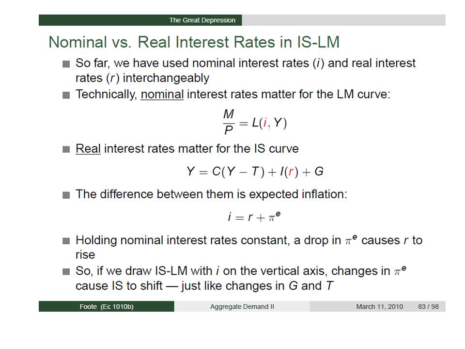
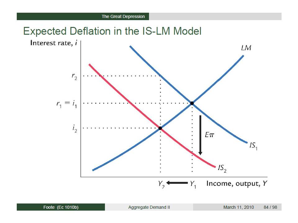
Scott asked me to list some monetary ideas that I believe are in conflict with IS-LM. I have done so in my earlier posts (here, here, here and here) on Earl Thompson’s paper “A Reformulation of Macroeconomic Theory” (not that I am totally satisfied with Thompson’s model either, but that’s a topic for another post). Three of the main messages from Thompson’s work are that IS-LM mischaracterizes the monetary sector, because in a modern monetary economy the money supply is endogenous, not exogenous as Keynes and Friedman assumed. Second, the IS curve (or something corresponding to it) is not negatively sloped as Keynesians generally assume, but upward-sloping. I don’t think Friedman ever said a word about an upward-sloping IS curve. Third, the IS-LM model is essentially a one-period model which makes it difficult to carry out a dynamic analysis that incorporates expectations into that framework. Analysis of inflation, expectations, and the distinction between nominal and real interest rates requires a richer model than the HIcksian IS-LM apparatus. But Friedman didn’t scrap IS-LM, he expanded it to accommodate expectations, inflation, and the distinction between real and nominal interest rates.

Scott’s complaint about IS-LM seems to be that it implies that easy money reduces interest rates and that tight money raises rates, but, in reality, it’s the opposite. But I don’t think that you need a macro-model to understand that low inflation implies low interest rates and that high inflation implies high interest rates. There is nothing in IS-LM that contradicts that insight; it just requires augmenting the model with a term for expectations. But there’s nothing in the model that prevents you from seeing the distinction between real and nominal interest rates. Similarly, there is nothing in MV = PY that prevented Friedman from seeing that increasing the quantity of money by 3% a year was not likely to stabilize the economy. If you are committed to a particular result, you can always torture a model in such a way that the desired result can be deduced from it. Friedman did it to MV = PY to get his 3% rule; Keynesians (or some of them) did it to IS-LM to argue that low interest rates always indicate easy money (and it’s not only Keynesians who do that, as Scott knows only too well). So what? Those are examples of the universal tendency to forget that there is an identification problem. I blame the modeler, not the model.

OK, so why am I not a fan of Friedman’s? Here are some reasons. But before I list them, I will state for the record that he was a great economist, and deserved the professional accolades that he received in his long and amazingly productive career. I just don’t think that he was that great a monetary theorist, but his accomplishments far exceeded his contributions to monetary theory. The accomplishments mainly stemmed from his great understanding of price theory, and his skill in applying it to economic problems, and his great skill as a mathematical statistician.

1 His knowledge of the history of monetary theory was very inadequate. He had an inordinately high opinion of Lloyd Mints’s History of Banking Theory which was obsessed with proving that the real bills doctrine was a fallacy, uncritically adopting its pro-currency-school and anti-banking-school bias.

2 He covered up his lack of knowledge of the history of monetary theory by inventing a non-existent Chicago oral tradition and using it as a disguise for his repackaging the Cambridge theory of the demand for money and aspects of the Keynesian theory of liquidity preference as the quantity theory of money, while deliberately obfuscating the role of the interest rate as the opportunity cost of holding money.

3 His theory of international monetary adjustment was a naïve version of the Humean Price-Specie-Flow mechanism, ignoring the tendency of commodity arbitrage to equalize price levels under the gold standard even without gold shipments, thereby misinterpreting the significance of gold shipments under the gold standard.

4 In trying to find a respectable alternative to Keynesian theory, he completely ignored all pre-Keynesian monetary theories other than what he regarded as the discredited Austrian theory, overlooking or suppressing the fact that Hawtrey and Cassel had 40 years before he published the Monetary History of the United States provided (before the fact) a monetary explanation for the Great Depression, which he claimed to have discovered. And in every important respect, Friedman’s explanation was inferior to and retrogression from Hawtrey and Cassel explanation.

5 For example, his theory provided no explanation for the beginning of the downturn in 1929, treating it as if it were simply routine business-cycle downturn, while ignoring the international dimensions, and especially the critical role played by the insane Bank of France.

6 His 3% rule was predicated on the implicit assumption that the demand for money (or velocity of circulation) is highly stable, a proposition for which there was, at best, weak empirical support. Moreover, it was completely at variance with experience during the nineteenth century when the model for his 3% rule — Peel’s Bank Charter Act of 1844 — had to be suspended three times in the next 22 years as a result of financial crises largely induced, as Walter Bagehot explained, by the restriction on creation of banknotes imposed by the Bank Charter Act. However, despite its obvious shortcomings, the 3% rule did serve as an ideological shield with which Friedman could defend his libertarian credentials against criticism for his opposition to the gold standard (so beloved of libertarians) and to free banking (the theory of which Friedman did not comprehend until late in his career).

7 Despite his professed libertarianism, he was an intellectual bully who abused underlings (students and junior professors) who dared to disagree with him, as documented in Perry Mehrling’s biography of Fischer Black, and confirmed to me by others who attended his lectures. Black was made so uncomfortable by Friedman that Black fled Chicago to seek refuge among the Keynesians at MIT.


About Me

David Glasner
Washington, DC

I am an economist in the Washington DC area. My research and writing has been mostly on monetary economics and policy and the history of economics. In my book Free Banking and Monetary Reform, I argued for a non-Monetarist non-Keynesian approach to monetary policy, based on a theory of a competitive supply of money. Over the years, I have become increasingly impressed by the similarities between my approach and that of R. G. Hawtrey and hope to bring Hawtrey’s unduly neglected contributions to the attention of a wider audience.

My new book Studies in the History of Monetary Theory: Controversies and Clarifications has been published by Palgrave Macmillan

Follow me on Twitter @david_glasner

Archives

Enter your email address to follow this blog and receive notifications of new posts by email.

Join 3,263 other subscribers
Follow Uneasy Money on WordPress.com