In my previous post, I argued that an accounting identity, which tells us that two expressions are defined to be the same, must hold in every state of the world, and therefore could not be disproved by any conceivable observation. So if I define savings and investment (or income and expenditure) to be the same thing, I am simply restricting my semantic description of the world, I am not restricting in any way the set of observable states of the world that conform to my semantic convention. An accounting identity therefore has no empirical content, which means that the accounting identity between savings and investment cannot explain the process by which a macroeconomic model adjusts to a parametric change in the model, traversing from a pre-existing equilibrium with savings and investment being equal to a new equilibrium with savings and investment equal.
In his paper, “The Foundations of the Theory of National Income,” which I am attempting to summarize and explain in this series of posts, R. G. Lipsey provides a numerical example of such an adjustment path. And it will be instructive to follow that path in some detail. The key point about this model is the assumption that households decide how much to save and consume in the current period based on the disposable income received in the previous period. The assumption that all receipts of the business firms are paid out to owners and providers of factor services at the end of each period is a behavioral assumption (not an accounting identity) that rules out any change in the retained earnings held by firms. If firms were accumulating financial assets, then their payments to households would not match their receipts. The following simple model reflects a one-period lag (known as a Robertsonian lag) between household earnings and household consumption.
C(t) = aY(t-1) (behavioral assumption)
I(t) = I* (behavioral assumption)
E(t) ≡ C(t) + I(t) (accounting identity)
Y(t) ≡ C(t) + S(t) (accounting identity)
Y(t) = E(t) (behavioral assumption)
Y(t-1) = Y(t) (equilibrium condition)
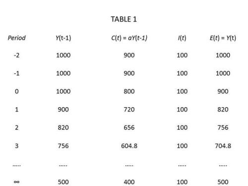
Assume that the economy starts off with a = .9 and I(t) = 100. The system is easily solved for E = Y = 1000, with C = 900 and I = 100. Savings, which is the difference between Y and C, is 100, just equal to I. The definition of saving will have to be fleshed out further below. Now assume that there is a parametric change in a (the marginal propensity to consume) to .8 from .9. This change causes equilibrium income to fall from 1000 to 500. By assumption, investment is constant, so that in the new equilibrium saving remains equal to 100. The change in income is reflected in a drop in consumption from 900 to 400. But given the one-period lag between earnings and expenditure, we can follow how the system changes over time, moving closer and closer to the new equilibrium in each successive period, as shown in the following table.
Consider the following questions.
First, in the course of this period-by-period adjustment, will there be any unplanned investment?
Second, in this example, the parametric change — an increase in the propensity of households to save — may be described as an increase in planned savings by households. Planned investment is unchanged. With planned savings greater than planned investment, will the household plans to increase savings be frustrated (implying positive or negative unplanned savings) as alleged in proposition 3 in the list of erroneous propositions provided earlier in the first installment in this series (see appendix below).
The answer to the first question is: not necessarily. There is nothing to prevent us from assuming that all firms correctly anticipate the reduction in consumer demand, so that production falls along with consumption with no change in inventories. It is not necessary to assume that firms can foresee the future; it could be that all consumption is in the form of services, or that production is undertaken only in response to consumer orders. With inventories unchanged, there is no unplanned investment.
The answer to the second question is that it depends on what is meant by unplanned savings. Unplanned savings could mean that households wind up saving an amount other than the amount that they had intended to save at the beginning of the period; households intended to save 200 at the beginning of period 0, but because their income turned out to be only 900, instead of 1000, in period 0, household savings, under the accounting identity, is only 100 instead of 200. However, households intended to consume 800 in period 0, and that is the amount that they actually consumed. The only sense in which households did not execute their intended plans is that household income in period 0 was less than households had expected. Lipsey calls this a distinction between plans in the point sense, and plans in the schedule sense. In this scenario, while plans in the schedule sense are carried out, plans in the point sense are not, because households do not end up at the point on their consumption functions that they had expected to be on.
So the equilibrium condition above that income does not change from one period to the next can be restated as follows: the system is in equilibrium when planned savings equals realized savings. Planned savings is the unconsumed portion of households’ expected income, which is the income households earned in the previous period. The definition embodies a specific behavioral hypothesis about how households formulate their expectations of income in the future.
S_p_(t) ≡ Y(t-1) – C(t).
Realized savings is the unconsumed portion of households’ actual income in the current period. It can be written as
S_r_(t) ≡ Y(t) – C(t).
Or restated differently yet again, the equilibrium condition is that actual disposable income in period t equals expected disposable income in period t.
Let’s flesh out the behavioral assumptions behind this model in a bit more detail. Business firms disburse income to households (owners and providers of factor services) at the end of each period. Households decide how much to save and consume in the upcoming period after receiving their incomes from firms at the close of the previous period. Savings are in the form of bond purchases made at the start of the period. Based on the consumption and savings plans formulated by households at the start of the new period, firms decide how much output to produce and how much labor to hire to produce that output, firms immediately notifying households how many hours they will work in the upcoming period. However, households are committed to the consumption plans already made at the beginning of the period, so they must execute those plans even if the incomes earned during the period are less than anticipated.
In our example, by choosing to increase their savings to 200 through bond purchases at the beginning of the upcoming period, while reducing consumption from 900 to 800, households cause business firms to reduce output from 1000 to 900 (investment being unchanged), and to reduce employment (measured in terms of total hours worked) by 11.1%. After buying bonds equal to 200, households have 800 left in cash, with which they finance their purchases for the rest of the month. So it is not obvious that households were unable to execute any of their plans during the period. However, at the end of the period, households receive only 900 in income from business firms, so although households did buy bonds equal to 200 at the start of the period, they carry over only 900 in cash into the next period, not 1000 as expected. Thus, realized savings are only 100 instead of 200, because household cash holding at the endo f the period turned out to be 100 less than expected. Nevertheless, it is difficult to identify any plan to save that was frustrated, inasmuch as households did purchase bonds equal to 200 at the beginning of the period, and did reduce consumption as planned. As Lipsey puts it:
[W]hether or not the actual real plans laid by households are frustrated depends on what plans households lay, i.e., it depends on our behaviour assumption, not on our definitions. If we assume that households make point plans about their bonds, and schedules plans about their transactions and precautionary balances, then no frustration of plans occurs.
If the statement quoted in (3) [see appendix below] is meant to have empirical content, it depends on a very specific hypothesis about households’ savings plans. These plans must be made in the point and not in the schedule sense, and the plans must include not only additions to the stock of income-earning assets, but also point-plans concerning transactions balances even though the household does not now know what level of transactions the balances will be required to facilitate. . . .
[W]e are now in a position to see what is wrong with statement (2), that actual savings must always equal actual investment, and statement (5), which draws the analogy with demand and supply analysis. Consider statement (2) first.
In the General Theory, Keynes stressed the fact that savings and investment decisions are made by different groups and that there is thus, no reason why planned investment should equal planned savings. [It has been argued] that, although plans can differ, actual realised saving must always be equal to actual realised investment, and, therefore, when planned savings does not equal planned investment, either the plans of savers, or of investors, must be frustrated. Of course, it is quite possible to define savings and investment so that they are the same thing, but it is a basic error to equate the magnitude so defined with the magnitude about which savers actually lay plans. Since ex post S and I as defined bear no relation to the magnitudes about which savers actually make plans, we can deduce nothing about what happens when ex ante S is not equal to ex ante I from the fact that we chose to use the terms ex post S and ex post I to refer to a single, and different, magnitude. The basic error arises from the assumption that households and firms make plans about the same magnitude when they are planning their savings and investment. The traditional theory defines investment as goods produced and not sold to households (= capital goods plus changes in inventories). According to our theory of the behaviour of firms, this is what firms do lay plans about: they plan to add so many capital goods and so many inventories to their existing holdings. The theory then says I ≡ S, and , thus, builds in the implicit assumption that households lay plans about the same magnitude. But according to the standard theory of household behaviour, they do not do so! Households, not subject to money illusion, are assumed to wish to lay aside a certain quantity of real purchasing power which is either used to increase the holdings of cash or used to purchase bonds. There is nothing in the standard theory of household behaviour that leads us to hypothesise that households care whether or not there exists – produced but unconsumed – a physical stock of goods which is the counterpart of the money they have laid aside. Indeed why should they? All they are assumed to care about is the potential real purchasing power of their savings, and this depends only on the amount of money saved, the present price level, and the expected future price level.
This is one of the keys to the whole present confusion: households lay plans about a magnitude that is different from the one that firms lay plans about. Firms plan to have produced and unconsumed a certain quantity of goods, while households plan to leave unspent a certain quantity of purchasing power. This means that it is quite possible for planned investment to differ from planned savings and to have both sets of plans fulfilled so that actual, realized investment differs from actual realized savings. [footnote: Now, of course, we mean by realised S and I the realised magnitudes about which firms and households are actually laying plans. This, of course, does not interfere with the statistician saying that realised savings is identical with realised investment since he refers to a different magnitude when he speaks of realised savings.]
Now consider another variation of the numerical example in Table 1. Instead of a change in the propensity to consume in period 0, assume instead that planned investment drops from 100 to 0. Starting with period -1, Table 2 displays the same initial equilibrium as in Table 1. Because we make a behavioral hypothesis that inventories do not change, planned and realized investment must be zero in period 0 and in all subsequent periods.
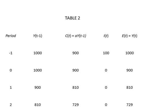
According to the national-income identities, savings must equal zero because investment is zero. But what is the actual behavior that corresponds to zero saving? In period 0, households carried over 1000 in cash from period -1. From that 1000, they used 100 to buy bonds and spent the remainder of their disposable incomes on consumption goods. So households planned to save 100 and consume 900, and it appears that they succeeded in executing their plans. But according to the national-income identities, they failed to execute their plan to save 100, and saved only 0, presumably because there were unintended savings of -100 that cancelled out the planned (and executed) savings of 100. So it appears that we have come up against something of a paradox. Here is Lipsey’s solution of the paradox.
[A]ny definitions are possible if consistently used, but this use of the word “unintended” has nothing to do with intended and unintended behaviour. To preserve the identity we must say that the plans of households were frustrated because a real counterpart of the saving they successfully made was not produced. We may say this if we wish, but the danger is that we will think we have said something about the world, and about the actual experiences of households. Indeed, a perusal of established textbooks shows that this confusion has occurred over and over again.
Thus, we conclude that, when we define investment as production not consumed, and savings as income [not consumed] . . . there is no reason why actual savings should not differ from actual investment.
Finally, what about the analogy between savings and investment in macro analysis and demand and supply in micro analysis as in erroneous statement (4) (see appendix)? If we write demand for some good as a function of the price of the good
D = D(p),
and write the supply of some good as a function of the price of the good
S = S(p),
then our equilibrium condition is simply D = S, where D represents desired purchases of the good, and S represents desired sales of the good. Because the act of selling logically entails the activity of purchasing, a purchase and a sale are merely different names for the same thing. So the plans of demanders to buy and the plans of suppliers to sell are plans about the same thing. The plans of demanders to buy and the plans of suppliers to sell cannot be fulfilled simultaneously unless there is an equilibrium in which demand equals supply. The difference between the microeconomic equilibrium in which demand equals supply and the macroeconomic equilibrium in which savings equals investment is that suppliers and demanders in a market are making plans about the same magnitude: sales (aka purchases) of a good. However,
in the national income case the two sets of real plans (savers’ and investors’) are laid about two different magnitudes. Thus the analogy often draw between the two theories in respect of plans and realized quantities is an incorrect one.
Appendix: List of Erroneous Propositions
1 The equilibrium of the basic Keynesian model is given by the intersection of the aggregate demand (i.e., expenditure) function and the 45-degree line representing the accounting identity E ≡ Y.
2 Although people may try to save different amounts from what people try to invest, savings can’t be different from investment; realized (ex post) savings necessarily always equals realized (ex post) investment.
3 Out of equilibrium, planned savings do not equal planned investment, so it follows from (2) that someone’s plans are being disappointed, and there must be either unplanned savings or dissavings, or unplanned investment or disinvestment
4 The simultaneous fulfilment of the plans of savers and investors occurs only when income is at its equilibrium level just as the plans of buyers and sellers can be simultaneously fulfilled only at the equilibrium price.
5 Whenever savers (households) plan to save an amount different from what investors (business firms) plan to invest, a mechanism operates to ensure that realized savings remain equal to realized investment, despite the attempts of savers and investors to make it otherwise. Indeed, this mechanism is what causes dynamic change in the circular flow of income and expenditure.
6 Since the real world, unlike the simple textbook model, contains a very complex set of interactions, it is not easy to see how savings stay equal to investment even in the worst disequilibrium and the most rapid change.
7 The dynamic behavior of the Keynesian circular flow model in which disequilibrium implies unintended investment or disinvestment can be shown by moving upwards or downwards along the gap between the expenditure function and the 45-degree line in the basic Keynesian model.

Needless to say I agree with David’s last blog on the identities matter. I wish only add two further points and one further illustration.
1. Everyone who comments further on this issue should commit themselves to saying TRUE or FALSE to the following statement: “Because definitional identities are consistent with all states of the universe, they cannot to be used to rule out any conceivable event.”
2. It should be obvious that one cannot do any dynamics with either the two sets of equations (i) E = A + cY and (ii) E ≡ Y or (iii) E = A +cY and (iv) E = Y. The former because (ii) is an identity and the latter because the two equations contain no dynamic elements. (iii) and (iv) do define an equilibrium position but not a dynamic process by which that equilibrium is reached. To do to this we need two things: (i) assumptions concerning the lags that exist in the dynamic adjustment process (there can be no dynamics if everything adjusts instantaneously) and assumptions about expectations.
The issues in dynamics were laid out in David’s summary of the argument in my paper. Here, however, is an even simpler example that makes the above points about dynamics and shows how the identities are preserved even when realised savings do not equal realised investment.
Consider a simple economy that produces only one good, C, all of which is initially consumed when the economy is in (neutral) equilibrium at Y = $100. There are 100 $1 bills that are used in the economy’s transactions. During each period $100 worth of C is produced and at the end of the period $100 is paid out to the households who are the producing agents. The households spend their $100 in the next period. (This is close to what really happens when we work to produce goods each week (or any other time period) and get paid at the end of the week and then spend the money over the next week.) This is an example of the type of lag we must have if we are to do dynamics.
Now let households plan to save 10% of the incomes starting in period t+1. In that period only $90 is spent on C and 10 $1 bills are put under mattresses. Now we must decide on the expectations of producers. There are two polar extremes: (i) they anticipate the sales that will be made in each period and produce only enough to satisfy demand; (ii) they assume that they will sell what they sold last period. First take the case of foresighted producers. In period t+1 they only produce 90 units of C and therefore generate only $90 of income to be spent in period t+2. In each subsequent period, production and income fall by 10% as income approaches its final equilibrium of zero. At this point, all 100 $1 bills will be under mattresses indicating $100 of savings but there will have been no inventory accumulation to act as investment.
We national income accountants do not deal with lags and so we will record $90 of income produced and earned in period t+1 and $90 of expenditure, $81 earned in t+2 and $81 spent and so on. So the identity is preserved while households actually save 10% of the income earned in the previous period.
In the second case, producers expect to sell what they sold last period and do not wish to hold any inventories. In period 2 they produce 100 but sell only 90 and so accumulate undesired inventories of 10. In the next period they expect to sell 90 and so only produce 80 expecting to sell their undesired inventories of 10. Following this through produces an interesting sequence with inventories slowly falling as firms sell a little more than they produce but less than they expect to sell from the sum of current production and accumulated inventories. Anyone interested can follow the sequence out and see how savings and investment in inventories never match after period t+1 while undesired inventory holdings slowly diminish as actual sales persistently exceed production plus current inventories while falling short of expected sales.
Morals: The attempt to infer dynamic behaviour from a static model is invalid; when needed dynamic assumptions are made all sorts of possible paths emerge as income converges on its equilibrium value. In all cases measured Y and E, calculated without time lags, will be identical while actual Y and E may diverge as may actual S and I.
Richard Lipsey
LikeLike
“An accounting identity therefore has no empirical content, which means that the accounting identity between savings and investment cannot explain the process by which a macroeconomic model adjusts to a parametric change in the model, traversing from a pre-existing equilibrium with savings and investment being equal to a new equilibrium with savings and investment equal.”
Yet to read your whole post, identities hold both in equilibirum and in the traverse. There may not be an equilibrium at all but identities hold.
More importantly it is misleading to say it has no empirical content and “cannot explain” because whatever model you use, you have to put the constraints (identities) and hence it restricts the outcomes.
More generally, I am really unsure about where you are headed. Do I throw away accounting identities and make models paying no attention to the identities?
LikeLike
First, to meet Richard Lipsey’s request, I will answer “TRUE”, based on my assumption of what he means. But we use definitional identities in models to establish the limitations of the model, so it’s not generally true to say they are consistent with all states of the universe. I can define my terms to describe a closed economy, but I can certainly conceive of an open economy. I know this is not what Lipsey means, but it is relevant, because it is the reason why we need definitional identities in these models.
I also agree with a lot of what you say, including that identities alone tell us nothing, nor do equilibrium behavioural conditions tell us anything about dynamic adjustment.
But adding in a bit more about behaviour will still let you look at dynamics. You don’t have to change the definitions. All you seem to be doing is choosing a different definition of saving and then demonstrating that it doesn’t necessarily equal investment. I was trying to understand what you were defining saving as actually being, but maybe Lipsey’s example helps.
Looking at his example, and taking the first instance where firms correctly anticipate sales, I note the comment that “…households actually save 10% of their income…” . As far as I can see here, households start with $100, they put $10 under the mattress, they spend $90 and receive $90 of earnings. So they end up with $100 – $10 under the mattress and $90 in hand – the same amount they started with, just in different places.
That to me means their actual saving is zero. Lipsey seems to be defining saving as only the cash put under the mattress, but that doesn’t seem very useful to me.
LikeLike
Nick: No one disagrees that we need to define our terms. And these definitions restrict the domain of our theory but they do not restrict anything that actually happens in the real world.
We can use words any way we wish in my example but people end up with $100 that ordinary people would call savings and there is no investment counterpart in terms of accumulated inventories. If you follow out my second example, you will see that inventories change in a way that is different from the income not spent on C in each period.
LikeLike
Richard,
I can see that people end up with 100 $1 bills with no counterpart in inventories, but that’s because they started with 100 $1 bills (It would be a fair question to ask where the bills came from in the first place, but we can probably let that pass). Their change in financial asset holdings (zero), exactly matches the change in inventories (zero). The only reason the stock of savings doesn’t equal the stock of inventories at the end is that they were not equal at the start.
If I look at your alternative scenario, I always have change in inventories equal to income less consumption, but I’m not sure what definitions you’re using there and under the definitions I’m using, they could never be different. Maybe by “the income” you mean the previous period’s income?
LikeLike
My take away from this great series of posts is that it is the behavioral assumptions that drive models not the accounting identities.
If the aim was to make one see why the “List of Erroneous Propositions” are indeed erroneous then I think I see that, but i do think most of them depend upon defining savings as “The amount allocated to a savings activity (like buying bonds or stuffing cash under the mattress)” rather than “The difference between income received and and consumption spending.”
Defined in the second way then planned savings and actual savings could differ but actual savings and actual investment never could, so most of the “Erroneous Propositions” become true.
From a conceptual POV both definitions of savings are useful. It is a shame that different names can’t be found for them.
LikeLike
“Because definitional identities are consistent with all states of the universe, they cannot to be used to rule out any conceivable event.”
my opinion is that the above statement is false
the identity forces framings of the plausibility of events which i may rank by likelihood or reject in a confidence region.
it clarifies what I must actually look at in an empirical world to reject my assumptions…which would be my understanding of falsifiability…and in this sense i think it is how it is used by people like Fama and Cochrane when they argue with Krugman over the power of the S=I identity…
LikeLike
I have a question on Richard’s model.
He says “inventories slowly fall[] as firms sell a little more than they produce but less than they expect to sell from the sum of current production and accumulated inventories.”. If savings is 10% of income, and income is based on production, won’t firms always sell less than they produce and cause inventories to grow ?
LikeLike
OK, I see how the model works now (“In each subsequent period, production and income fall by 10% as income approaches its final equilibrium of zero”).
But while “Anyone interested can follow the sequence out and see how savings and investment in inventories never match after period t+1” is true if you define savings as “$1 bills are put under mattresses” , but it is not true if you define it as “the difference between Y and C” (which it always is).
LikeLike
This is, as ever, very interesting to a non-economist like me. Thanks for the example which makes what you are saying much easier to understand. It seems like there are two different topics here. The first topic is accounting identities. The second topic is planning and how planning discrepancies between different parties can cause problems. I’d suggest that the second topic can only be discussed properly when any issues on the first topic have been resolved, so I’m only going to comment about the accounting identities.
I have two issues with your example with reference to the identities. They both relate to the purchase of bonds by households but are really about the definition of terms and the rules of accounting. I’ll discuss the first issue in this comment and the second in a separate comment.
My first issue concerns the definition of Saving and whether it includes or excludes bonds. This may be obvious to economists but it is not clear to non-economists so I will try to argue pedantically from first principles.
The only sensible answers are: yes Saving does include bonds or no it does not. Let’s take each in turn.
First, assume that bonds ARE included in saving (I think that this is your definition):
Saving (Total) = Saving (Money) + Saving (Bonds) + Saving (Other)
In this case, when households buy 200 bonds,
Saving (Total) = Saving (Money – 200) + Saving (Bonds + 200) + Saving (Other)
Hence, there is no change to the overall value of Saving (Total), just a change in the composition of the saving.
In this case, the only real net saving relevant to the identity seems to be the -100 of saving due to the shortfall in income, so your conclusion about realisation of plans seems to be wrong.
This definition also raises the question for non-economists of what else might economists be including in household saving. Why are bonds considered to be saving and not property, jewellery, cars or many other things? All of these things have value. All of them can be purchased with money. All of them can be resold. All of them might rise or fall in value. What makes bonds special? Economists never seem to answer this question unambiguously.
Second, assume that bonds ARE NOT included in saving (I don’t think this is your definition but it is logically consistent if bonds are not viewed as special):
Saving (Total) = Saving (Money)
In this case, when households buy 200 bonds,
Saving (Total) = Saving (Money – 200)
Hence, Saving (Total) reduces by the 200 spent on the bonds.
In this case, the saving relevant to the identity is the -200 from the bond purchase plus a further -100 due to the shortfall in income, so your conclusion about realisation of plans again seems to be wrong.
This definition also raises the question of how we account for the value of the bonds that were purchased. That’s a very good question but it is also a very good question for purchases of everything else including property, jewellery, cars etc. Economists never seem to answer this question unambiguously either.
David said: “Savings are in the form of bond purchases made at the start of the period”
David said: “The only sense in which households did not execute their intended plans is that household income in period 0 was less than households had expected. Lipsey calls this a distinction between plans in the point sense, and plans in the schedule sense. In this scenario, while plans in the schedule sense are carried out, plans in the point sense are not, because households do not end up at the point on their consumption functions that they had expected to be on”
If bonds are included in saving (which seems to be your assumption based on the first quote) then “plans in the schedule sense” are the bond purchases which, as I argued earlier, are offset by dissaving the money used to buy the bonds. “Plans in the point sense” are the only real net saving. These plans are achieved only because they are not really plans. ‘Point sense’ seems to mean ‘save whatever is left over by default’.
LikeLike
My second issue is more fundamental. Accounting is based on the fact that things are conserved, so your example raises the question of where the purchased bonds come from. I will assume that bond holdings are included in the definition of household saving.
If households purchase existing bonds from each other then purchases and sales will cancel out. Given that there is a net household purchase of 200 bonds in your example then those bonds must be ‘manufactured’ somewhere else. Let’s assume that the government issues the bonds. Something like the following must occur.
Start position:
Government: Investment (0)
Households: Saving (Money)
Government ‘manufactures’ 200 bond assets and equal and opposite 200 bond liabilities ‘out of nothing’. Position changes to:
Government: Investment (200 bonds as asset) + Investment (200 bonds as liability)
Households: Saving (Money)
Now, the households buy the 200 bonds as per your example. Position changes to:
Government: Investment (200 bonds as liability) + Saving (200)
Households: Saving (Money – 200) + Saving (200 bonds as asset)
Presumably, the government issues the bonds so that it can use the money to fund spending (resulting in additional demand for businesses) or to fund some sort of transfer back to households. Let’s keep it simple and assume a transfer back to households. Now, position changes to:
Government: Investment (200 bonds as liability)
Households: Saving (Money) + Saving (200 bonds as asset)
Hence, household saving increases by 200 bonds over what it would have been if the bonds had not been issued. However, that increase in saving comes from the combination of the bond purchase AND the government transfer.
I’m not a finance guy so there may be a more elegant way of expressing this. However, the key message is that households can’t buy bonds unless those bonds come from somewhere. Your example doesn’t explain where the bonds come from, or what the bond issuer does with the funds it receives for selling the bonds, so your accounting seems to be incomplete.
A similar argument would also apply if businesses issue the bonds but, presumably, businesses would use the additional funds to buy things from other businesses (resulting in additional demand for the other businesses).
LikeLike
Excellent series in total.
Sensible people should really agree that accounting does not explain behavior. That should not be the issue. But it seems to be a straw man often presented by those who are defensive about the relationship between accounting and economics.
Accounting in fact does depict the evolution of economic transactions that result from behavior. And there is an issue of holistic coherence in that relationship as it pertains not only to ex post measurement, but to ex ante modelling of realizable behavior in total.
The approach in general in this series (a la Glasner/Lipsey) seems rooted in a pessimism about the capability of economic agents to undertake coherent financial planning. I find that disturbing. Financial planning intersects with economics, but economics is not a monopoly authority on the subject.
It seems that the behavioral assumption is that agents are incapable of distinguishing between the concept of a balance sheet and the concept of an income statement. As an illustrative example, we are asked (to take an representative case) to assume that agents mistakenly deceive themselves into thinking that they have automatically saved for 2015 by purchasing bonds using a bank balance that existed on New Year’s Eve.
I find it unrealistic that agents are assumed to be generally incapable of imagining a desired change in their wealth position from January 1 2015 to December 31 2015. Because if they imagine such a change, then they will have considered the contribution of saving from 2015 income in the larger context, that context being the change in balance sheet position over the time period in question. And they will not deceive themselves into thinking that because that they bought bonds on January 1 using a bank balance that existed on December 31 that they will have automatically saved correspondingly for 2015. People are not that dumb. They may not do precise projections, but they know things can happen that may cause their wealth position in total to be less than what they would like it to be in the future. They are capable of recognizing the difference between buying a bond on January 1 – which in and of itself has no net effect on their wealth position – and having successfully saved some amount of their income over the course of 2015 by the time the year is over.
And once it is allowed that agents are capable of imagining a change in their balance sheet position over a given time period, it quickly follows that planning for saving is entirely congruent with planning for investment at the macroeconomic level. This is just making the logical connections in adding up micro accounting to macro accounting, plus the fact that accounting identities – which exist now and which have existed in the past – will continue to exist in the future.
Instances of accounting confusion obscure what should be standard logical connections between balance sheet, income statement, and flow of funds (sources and uses of funds) accounting. This detracts from a more accurate understanding of how behavioral results ex post (as well as future possibilities) should be seen as a sequence of economic transactions with a coherent record of account. An interpretation of economic behavior that is premised on household financial illiteracy/innumeracy seems somewhat disturbing as a model feature.
LikeLike
David,
“Households decide how much to save and consume in the upcoming period after receiving their incomes from firms at the close of the previous period. Savings are in the form of bond purchases made at the start of the period.”
The purchase of a bond with a pre-existing cash balance (prior period existing) is a flow of funds and nothing more. Households have notional income statements, and this sort of transaction does not appear as part of the income statement. It is completely independent of whether or not income or saving occurs in the current period. It is simply an asset allocation decision.
“Nevertheless, it is difficult to identify any plan to save that was frustrated, inasmuch as households did purchase bonds equal to 200 at the beginning of the period, and did reduce consumption as planned.”
Households would have to be assumed to be completely in the dark about how to interpret their own financial position, with no idea about the difference between an income statement and a balance sheet or just about anything else financial.
“But according to the national-income identities, they failed to execute their plan to save 100, and saved only 0, presumably because there were unintended savings of -100 that cancelled out the planned (and executed) savings of 100. So it appears that we have come up against something of a paradox.”
I see no paradox. It seems straightforward. Again, a household that has any idea of the concept of net worth and the effect on net worth of saving from income will be able to understand that its plans have not been realized.
LikeLike
Richard Lipsey,
“During each period $100 worth of C is produced and at the end of the period $100 is paid out to the households who are the producing agents. The households spend their $100 in the next period.”
This process starts somewhere. If it starts in period 1, it means that period 1 closes with an outstanding stock of inventory investment in an amount equal to C. In fact, what would have been C becomes I, because C was not sold during the period:
In other words, final period 1 accounting for the economy looks like this:
Y = 100
I = 100
S = 100
C = 0.
Y = C + I = C + S.
Consider period 2. Divide it into two parts.
In the first part of period 2, households consume from the outstanding stock of inventory investment that was established at the close of period 1. That consumption constitutes negative investment as a flow.
The economy’s income statement for the first part of period 2 immediately after the opening then looks like this:
I = (100)
S = (100)
C = 100
Y = 0 = C + I = C + S
Then, the economy produces output of 100, which becomes inventory investment as a flow. The income statement for the second part of period 2 looks like this:
I = 100
S = 100
C = 0
Y = 100 = C + I = C + S
Now add both of these sub-periods together and the full period 2 result is:
I = 0
S = 0
C = 100
Y = 100 = C + I = C + S
Because the full period flow of I is 0, the outstanding stock of inventory investment remains 100 just as it was at the end of period 1. This accounting holds for all periods up to and including period t.
Period t + 1 Case 1 (correct foresight):
“First take the case of foresighted producers. In period t+1 they only produce 90 units of C and therefore generate only $90 of income to be spent in period t+2. In each subsequent period, production and income fall by 10% as income approaches its final equilibrium of zero. At this point, all 100 $1 bills will be under mattresses indicating $100 of savings but there will have been no inventory accumulation to act as investment.”
My interpretation of this is that from period t + 1 forward there is no inventory investment accumulation as a flow and that correspondingly there is also no saving as a flow.
Here is the sequence as I visualize it starting in period t + 1:
At the opening of period t + 1, households consume most of the outstanding stock of inventory investment, but not the full stock as before. The economy’s income statement for the first part of period t + 1 immediately after the opening then looks like this:
I = (90)
S = (90)
C = 90
Y = 0 = C + I = C + S
Then, the economy produces output of 90, which becomes inventory investment as a flow. The income statement for the second part of period t + 1 looks like this:
I = 90
S = 90
C = 0
Y = 90 = C + I = C + S
Now add both of these sub-periods together and the full period t + 1 income statement is:
I = 0
S = 0
C = 90
Y = 90 = C + I = C + S
Because the full period flow I = 0, the outstanding stock of inventory investment at the close of period t + 1 remains 100, just as it was at the close of all prior periods. The difference now is that the outstanding stock of inventory at the end of period t + 1 consists of 10 held over as it existed at the close of period t and 90 that has been replaced from what was disinvested at the start of period t + 1.
Similarly, in subsequent periods, income and its components decline as per the model, but the outstanding stock of inventory investment remains the same. It just gets “older” due to the shrinking disinvestment/reinvestment component.
As far at the $ 100 bills are concerned, these bills exist as the form of cumulative saving at the end of all periods, offset by the outstanding stock of cumulative inventory investment. Both the $ 100 bills and the cumulative investment are stocks in place at the close of each period.
The original saving and investment flow of 100 was done in the first period. There is no net flow of investment or saving after that – only the continuation of stock balances. So period flows of 0 for investment and saving match up according to accounting identities.
At the conclusion of the process, the outstanding stock of cumulative investment and saving is the same as it was for the balance sheet at the end of every period – it is 100. It’s just that the level of income and consumption has declined in steps, while periodic investment and saving flow has held constant at 0.
So everything is in balance according to accounting.
Period t + 1 Case 2 (incorrect foresight) is a variation on the general theme. However, there seems to be an inherent contradiction in the specification of this alternative. Which is that if at the beginning of each period households buy consumer goods from the stock of the previous period’s closing inventory position, then producers know right away how their planned current period production will compare to current period consumption. So there is some foresight with respect to the expected current period result.
For example, if households consume 90 at the beginning of period t + 1, then producers know what the net effect of their production will be on closing inventories for period t + 1.
However, this case can allow for a sequence of periodic planning for declining closing inventory positions in response to the emerging sequence of declining consumption. For example, if t + 1 consumption is 90, then producers might produce 80 with the objective of reducing their closing inventory to 90. This pattern is somewhat similar to your Case 2 sequence, but it explicitly incorporates periodic closing inventories as I previously described. The producer has the option of managing that sequence of closing inventory levels down – as the result of knowing the current period consumption at the beginning of the period and using that knowledge in the current period production decision.
So period t + 1 starts out as in the first case:
I = (90)
S = (90)
C = 90
Y = 0 = C + I = C + S
Then, in an attempt to manage down inventory levels, the economy produces output of 80 in the second part of period t + 1, which becomes inventory investment as a flow. The income statement for the second part of period t + 1 looks like this:
I = 80
S = 80
C = 0
Y = 80 = C + I = C + S
Now add both of these sub-periods together and the full period t + 1 income statement is:
I = (10)
S = (10)
C = 90
Y = 80 = C + I = C + S
And the closing stock of inventory investment (and the stock of cumulative saving) has declined from 100 to 90 at the end of period t + 1.
And so on.
LikeLike
Richard, Thanks, as always, for your comment and further elucidation of the principle that a dynamic adjustment process requires some lags which are not accommodated by conventional income accounting.
Here is the issue that occurs to me with your new example. You explicitly introduce a quantity of money held fixed at 100 into the example, which I think is helpful. At the end of the adjustment when the economy reaches zero, all 100 is held by households with income, expenditure, consumption, investment and savings are all at zero. At the initial equilibrium, who was holding the money? Apparently at the end of each period in the initial equilibrium, 100 was paid by firms to households, so households start and period with 100 in cash, which is returned to them at the end of each period.
When households reduce spending, they spend only 90 and keep 10, but they still end up with 100 at the end of the period, so in what sense can it be said that they have succeeded in saving 10 by spending only 90? They tried to save 10, but the unexpected fall in income of 10 somehow prevents the intended accumulation of assets. I guess the difference is that at end of the adjustment, they will have 100 to spend even though their income in the period is zero, while in the initial equilibrium what is available for spending is equal to their income not their accumulated assets.
Ramanan, The nature of an identity is that it must always hold, otherwise it would not be an identity. The question is what inferences are we allowed to draw from the identity. It seems to me that the point is not to throw away the identities, but to be clear about what the identities are telling us and not telling us.
Nick, In the standard model with a government sector, the I ≡ S identity becomes an I + G ≡ S + T identity, when the model changes the corresponding identity changes. Both identities can be derived from the E ≡ Y identity.
As I pointed out above, it is meaningful to say that households have in fact saved over the course of the traverse to the new equilibrium, because in the new equilibrium with zero income, they would be able to spend 100 even though their income is zero.
In Richard’s example in which the reduction in consumption is associated with unintended inventory accumulation, when consumption drops to 90 in period 0, the receipts of firms are only 90 so that income in period 0 is 90 even though output was 100. There is unplanned investment of 10, corresponding to savings of 10, but household income is only 90, which is what business firms pay to households at the end of the period. So output equals 100, but expenditure only equals 90 and income only equals 90. If you count unplanned investment as expenditure, then expenditure is greater than income because households do not receive income for unplanned inventory accumulation. That’s how I am looking at it
.
I am pressed for time now and will try to respond to the remaining comments later this evening.
LikeLike
Rob, I think the different possible meanings of savings are only one of the possible reasons for why the erroneous propositions are erroneous. There are other possible reasons as well.
LAL, Tell me more about what Fama and Cochrane are arguing with Krugman about.
Rob, Whether inventories change unexpectedly depends on whether producers can predict what happens to demand, or, alternatively, whether they produce to order or produce to stock and sell from stock. If firms always predict demand correctly their inventories will not change unless they want them to change. Alternatively, if they only produce in response to having an order placed, there is no reason for inventories to change unless the change is desired.
Again, neither Richard nor I is insisting that savings can only be defined in one way.
Jamie, There is nothing special about bonds, spending money on any asset, not currently produced, e.g., land, works of art, etc., would also qualify as savings. According to some, even spending on consumer durables would qualify (in part as saving). Bonds are just a convenient way of categorizing saving. You are right that holding money, rather than spending it, would also be saving, so from that point of view, there is no difference between holding money or buying bonds. You are also right to point out that the bonds must come from somewhere, so in that respect, I agree that the model is not fully closed. But I think all those issues are avoided in the example provided by Richard in his comment which focuses entirely on saving by holding cash.
JKH, I think that you may not be grasping what, following Richard Lipsey’s lead, I am trying to argue in this series. I am not making a substantive argument on behalf of any of the models that I have been discussing. I believe that the simple income-expenditure model we have been talking about (aka the Keynesian cross) is woefully inadequate as an explanation of reality, and the assumptions underlying it are high unrealistic and unsatisfactory. I am not really sure if Richard Lipsey’s opinion of the model is as unsympathetic as mine; it might be marginally less negative, but I don’t want to speak on his behalf. The point is really not about the theory but about the metatheory. What are we really saying when we use the terminology of the income-expenditure model? I am trying to point out that any substantive statements about the real world that come out of the model, statements that are very often empirically wrong, are derived from assumptions about how people behave, not about the meaning of terms like savings and investment.
Having said that, I don’t think that your criticism of the behavioral assumption of the model that it assumes that people are “incapable of imagining a desired change in their wealth position” is relevant. What the model shows is that the wealth position of individual agents is determined not by their individual choices about how much to save or how much wealth to accumulate, but by their collective decisions. The model says that the attempt to accumulate wealth by restricting consumption is self-defeating (aka the paradox of thrift). That conclusion is not the implication of some misunderstanding of financial planning by individuals, but is the result of the behavioral assumptions and interactions among the relevant variables (savings, investment, income and expenditure) of the model.
I still have to work through your detailed numerical discussion of Richard’s example. Perhaps Richard will have comments on it before I do (I hope so). At any rate, I will try to have a response for you tomorrow.
LikeLike
JKH, I am sorry but I don’t understand at all what you are getting at in your response to Richard. You begin by saying:
“This process starts somewhere. If it starts in period 1, it means that period 1 closes with an outstanding stock of inventory investment in an amount equal to C. In fact, what would have been C becomes I, because C was not sold during the period:”
You seem to be referring to the initial equilibrium in Richard’s example. In the initial equilibrium all expenditure and income is devoted to consumption with zero saving and zero investment and no inventory is accumulated or held by business firms. I don’t understand why you want to divide the period into two parts.
You say:
“At the conclusion of the process, the outstanding stock of cumulative investment and saving is the same as it was for the balance sheet at the end of every period – it is 100. It’s just that the level of income and consumption has declined in steps, while periodic investment and saving flow has held constant at 0.”
At the end of the process there is no stock of inventory, but there is cash equal to 100 in the pockets (or mattresses) of households, with zero output, expenditure, income, consumption, investment and savings.
You also seem to misunderstand Richard’s incorrect foresight case.
You say:
“if at the beginning of each period households buy consumer goods from the stock of the previous period’s closing inventory position, then producers know right away how their planned current period production will compare to current period consumption.”
Producers at the beginning of the period decide how much to produce before knowing what household demand is; they simply guess that households will buy as much as they did in the previous period. Once they make their production plans they carry them through, even after they observe how much households are actually buying.
You may not like those assumptions, but those assumptions have nothing to do with the accounting identities.
LikeLike
David,
This really just comes down to choice of definitions. In your main post you say:
“The assumption that all receipts of the business firms are paid out to owners and providers of factor services at the end of each period is a behavioral assumption (not an accounting identity) that rules out any change in the retained earnings held by firms.”
The only reason Y(t) = E(t) is not an identity in your model is that you are using the terms in a different way. The income that we mean when we talk about it being identically equal to expenditure is the combined income of households and firms. That must still hold as an identity in your model. The income in your behavioural equation is just the income of households, and clearly that can differ from expenditure.
From your reply to me: “If you count unplanned investment as expenditure, then expenditure is greater than income because households do not receive income for unplanned inventory accumulation.”
If “income” includes income of firms, as is usual, then income and expenditure are equal.
I should say that I share your dislike of Sumner’s line of reasoning – I just don’t think this is the way to counter it.
LikeLike
David,
I’ll come back on your first response later on.
Regarding your reading of my summary of Richard’s model:
“You seem to be referring to the initial equilibrium in Richard’s example.”
No. I’m specifying what the accounting sequence must be – given that the model states that households don’t spend this period’s income until the next period, and given that the process must have started somewhere. There must be an inventory accumulation at the outset, or somewhere along the line, or Richard’s lag process can’t get started. Otherwise, there is a contradiction, because if there is no original inventory accumulation, or no accumulation at some point, the lag can’t get started.
“At the end of the process there is no stock of inventory”
Yes there is. Beginning with the point I just made, the accounting shows how it must be the case. The splitting of accounting periods into two parts is part and parcel of that explanation.
“They simply guess that households will buy as much as they did in the previous period.”
I understand Richard’s incorrect foresight case. However, I made the simplifying assumption that the previous period’s closing inventory was purchased right at the opening of the next period. That’s not a necessary assumption. So you have a fair point. My observation is correct given my assumption, but I could have relaxed the assumption. But it’s not an important point in the context of the overall accounting or its interpretation.
LikeLike
Nick, But the income that matters for the consumption of households is the income of households not the income of firms. It’s only from the payments firms make to households that households are able to spend. That at least is a possible behavioral assumption.
JKH, Richard’s lag process is based on a steady state equilibrium. There may well have been an earlier period in which there was inventory accumulation and the decumulation before the steady state was reached, but the analysis does not require that we go back to the beginning of time. It merely requires specifying some steady state equilibrium with an assumed lag structure.
LikeLike
David,
The accounting sequence does not require going back to “the beginning of time”.
In fact it assumes a finite starting point that is logically consistent with the assumed lag outcome. That requires a net inventory accumulation.
LikeLike
…
Assume zero net inventory accumulation. That means that in some period in the past, some output must have been purchased in the same period it was produced. Otherwise, there would be inventory accumulation. But the model specifies that periodic output is always purchased in the following period. So the assumption of zero net inventory accumulation is a contradiction.
Similarly, assume net inventory accumulation is positive but less than the steady state periodic output. Again that means that in some period in the past, some output must have been purchased in the same period it was produced. Otherwise, inventory accumulation would be equal to the steady state output. And that similarly is a contradiction.
So the assumption of any level of net inventory accumulation less than the periodic steady state output is a contradiction. Similarly, one can work out the conclusion that net inventory accumulation can’t be greater than the periodic steady state output. Therefore it must be equal.
The periodic structure of the model implicitly specifies the required periodic accounting result that corresponds to the model. That’s just what the model says – I didn’t specify the model.
LikeLike
David,
I agree with that and I have no problem with your model. It’s just that what you call Y, I think of as household disposable income, rather than income.
LikeLike
JKH, You wrote:
“the model specifies that periodic output is always purchased in the following period. So the assumption of zero net inventory accumulation is a contradiction.”
This seems to be the point on which we are not clear. As I understand the model, there is a one-period lag between the earning of income and the spending of income, but there is no lag between the production of output and the purchase of output. If there is no lag between the production of output and the purchase of output, why must there be any inventory accumulation?
Nick, In this model, income and disposable income are assumed to be equal, so there is no reason to distinguish between them.
LikeLike
David,
Richard says:
“During each period $100 worth of C is produced and at the end of the period $100 is paid out to the households who are the producing agents. The households spend their $100 in the next period.”
I guess the overriding point I would make is that there is a difference between income accounting and sources and uses of funds accounting (flow of funds at the macro level), and that this is worth bearing in mind throughout this exercise.
From a periodic income accounting perspective, there really is no such thing as a lag between income and expenditure. Current period income must equal current period expenditure. This is an income accounting tautology. The question in the simple model is whether the expenditure is on consumer goods or investment goods. If it is on investment goods, there is also saving as it is defined in income accounting.
The apparent dilemma of the lag in Richard’s example is captured in flow of funds accounting. If that $ 100 ends up as a bank deposit (or in dollar bills – the difference isn’t an issue) at the close of the income accounting period, it must show up on a household balance sheet as such.
Clearly that particular increase in the bank balance corresponds to income earned in the current period, and that income corresponds to output produced in the current period. Cost accounting for the output assures that it is matched up to income earned by the factors of production. But that income by assumption is not used to purchase final output in the current period. So I think it must represent income that is saved by definition. And that must correspond to inventory investment in the simple model. But I qualify all this by acknowledging that this only accounts for events in the latter part of the current period.
I offset this with inventory liquidation at the front end of the current period – as per the steady state flow of funds, since the delay until next period in spending the cash balances attributable to income earned in the current period was preceded by the same type of delay in making the transition from the previous period to the current period.
If there is no inventory accumulation in the latter part of the current period, then I’m not sure how the bank balance can correspond to the payment to the factors of production that produced the current period output. And how does one explain the presence of that positive bank balance, if it does not represent saving in the second half of the period? And how does one explain that saving if it does not correspond to inventory accumulation?
Thinking about all this gets a bit circular, but this is what I keep coming back to. It is premised on the fact that output (and expenditure) must equal income in periodic income accounting.
Obviously the real world is more complicated than this. The pattern of inventories is much more complex due to the effect of the sub-periodicity of comparable funds flows within given accounting periods, the effect of consolidating many such overlapping patterns for the entire economy, and the effect of the banking system’s ability to pre-fund such flow of funds lags at the margin. But this is just what the simple model described by Richard tells me, including the way in which I regressed it back. (I’m not sure what you described in your post is quite the same but I haven’t reexamined it as closely.)
I think I understand the effect of flow of funds lags as they impacts on behavior in your models. But I don’t think income accounting needs to be upset in demonstrating how this can happen. Double entry bookkeeping can handle any realizable economic outcome, while preserving the equivalence of realized investment and realized saving in a given accounting period.
P.S.
Just a side point on the Keynesian Cross. I’ve always been suspicious of that vertical gap between the 45 degree line and the AD/planned expenditure line where the first is higher than the second. That gap is depicted as corresponding to unplanned inventory accumulation I believe. But in fact the actual path of the economy’s adjustment must be rolling down the 45 degree line. And that is a continuous line. What that means to me is that the AD line itself as a single line cannot represent the process accurately. The process is really an iteration down through similar lines that are stacked on top of each other in effect, as the economy ripples through a sequence of near term AD lines before reaching the original lowest one which is more like a final objective or plan, as opposed to a “jump” process that is associated with any realized quantity of near term inventory accumulation. The inventory process will be iterative as the economy starts the adjustment process in other sectors with other changes that complement that of the inventory process, but it will not be a single jump change as represented in the KC model (as I understand it).
LikeLike
David said: “But I think all those issues are avoided in the example provided by Richard in his comment which focuses entirely on saving by holding cash”
Richard had said previously: “Now let households plan to save 10% of the incomes starting in period t+1. In that period only $90 is spent on C and 10 $1 bills are put under mattresses”
If I’ve understood correctly, I think that Richard is making the same mistake. He is assuming that “10 $1 bills are put under mattresses” is saving i.e. saving is an action. However, saving is not an action. “Putting under mattresses” is not saving. In order to put money under mattresses, you need to have that money in the first place. The increase in saving occurs when you obtain the money in the first place i.e. when you are paid your wages. After that point you can choose to spend some of your money – which will reduce your savings, or you can choose not to spend your money – which will not reduce your savings. “Putting under mattresses” is just an example of not spending. “Taking out from under mattresses” is the exact opposite of “putting under mattresses” but you don’t have any less savings just because you move the money from under mattresses to your hand.
In Richard’s case, if I’ve understood correctly, people are paid at the end of a period. That means that their saving of that period’s wages takes place at that point i.e. in that period. In the next period, they spend less money and receive corresponding less wages. The “putting under mattresses” is not relevant.
David said: “According to some, even spending on consumer durables would qualify (in part as saving)”
Yes, I think that, “according to some” economists, you are correct here. However, that is my problem as a non-economist. There is no consistent view of what is saving amongst economists and, so, there is no consistent logic involved in the definitions in the accounting identity. It’s the absence of consistent and logical definitions that causes all of the problems with this stuff. After the definitions get out of synch between people, all further discussion is at cross purposes.
I am going to try to answer the challenge you put in your next post. However, I need to look out some diagrams first. I will put forward a view in that comment that saving is just the accumulation of money and that all spending is consumption, and I will try to show why that is the most logical definition.
LikeLike
JKH, You said:
“From a periodic income accounting perspective, there really is no such thing as a lag between income and expenditure. Current period income must equal current period expenditure.”
Are you saying that it is impossible for households to receive income at the end of the period in which they provide services to business firms and to use the income earned in (and received at the end of) the previous period to finance their expenditures in the next period? If so, your accounting identities do have empirical content, and they are refuted. That’s what living paycheck to paycheck means.
It is fine to say that income received at the end of the period is saved, but, in equilibrium, the saving at the end of the period only offsets an equal amount of previous dissaving during the period of income received at the end of the previous period which was used to finance consumption in this period. Total saving in the period is zero, and there is no – and there cannot be any — inventory accumulation because all output is, let’s assume, made to customer order at the beginning of the period and delivered to – or picked up by — the customer upon completion.
Forgive me, but I can’t penetrate what you are saying about the Keynesian cross, and, in any event, it seems like a side issue which I am too far behind to try to figure out.
Jamie, I think you are completely missing the point. Saving is passive. It occurs when households leave some of their income unspent. That is the saving. I think it is perfectly ok to call that an act of saving, by the way; it is a commonplace to speak of “acts of omission.” Putting unsaved income under the mattress is just one way of disposing of the savings. So you are just caught up in a semantic muddle of your own making.
LikeLike
David,
First:
“Are you saying that it is impossible for households to receive income at the end of the period in which they provide services to business firms and to use the income earned in (and received at the end of) the previous period to finance their expenditures in the next period? If so, your accounting identities do have empirical content, and they are refuted. That’s what living paycheck to paycheck means.”
Yes, that is what I am saying in the sense of describing what happens using correct, coherent accounting. And the right accounting relationships reflect empirical events perfectly. That’s what accounting does. It systematically classifies and records stuff that happens.
Income is a periodic accounting concept. A period’s income pertains to that period. Once the books are closed for that period, that income is history.
In this case, the household saves the income it received in the second part of period t, according to how I depicted the partitioning of each period into two parts. That flow of saving in the second part of period t results in a stock of balance sheet savings at the end of the period. That is what I have described. The income story for that period is now finished.
In the first part of period t + 1 the household uses that stock of savings (in the form of a bank balance in my example) to acquire consumer goods from the closing inventory of the previous period.
That transaction on its own reflects dissaving for the first part of period t + 1. It does not directly represent the spending of current period income, because current period income will be reflected fully according to additional information on what happens later on in the period. It represents a flow of funds from the bank account of the household to the bank account of the firm. For the moment, that dissaving is offset by the value of the consumption good received in exchange. But because that consumption good by definition will be consumed in the current period, the net result of that transaction is dissaving in the first part of period t + 1.
This is why I split the analysis into two sub-periods. In the second part of the period, we can account for the income received in the period. That income is saved in the second part of the period by assumption, and is equal to the value of the production of new inventory investment in the period. That accounts for the income received in the current period. It cannot be used in the next period or any other accounting period.
Add the two parts together, and the result for the current period in its entirety is consumption equal to income with net saving of zero. And net investment is zero for the period because inventory disinvestment (with negative saving) at the front end has been offset by inventory investment (with saving) at the back end.
Nowhere is income from the previous period used to acquire goods in this period. It is the opening stock of savings that is used to acquire the inventory that was the output of the previous period. The relevant flow of funds results in the exchange of a savings stock for an inventory stock.
Anticipating the possibility that there may be a suggestion of semantics at play, instead the distinction here is important for the topic under discussion. It is important because to ignore it is to tempt the kind of accounting confusion that leads to the construction of incoherent accounting stories. And the notion of attempting to disprove correct and coherent accounting relationships by getting them wrong in the first place is a nonstarter. Everything depends on everything else in coherent accounting.
So, in short, last period’s income is used in the last period. This period’s income is used in this period. That is the meaning of the correct accounting.
Any overlap of activity or connection of activity between two periods must be explained using flow of funds accounting and balance sheet accounting – not accounting that attempts to confuse the income received in two different periods as if used within a single period.
And this principle holds whether at micro accounting or macro accounting levels.
Now, this piece:
“It is fine to say that income received at the end of the period is saved, but, in equilibrium, the saving at the end of the period only offsets an equal amount of previous dissaving during the period of income received at the end of the previous period which was used to finance consumption in this period. Total saving in the period is zero, and there is no – and there cannot be any — inventory accumulation because all output is, let’s assume, made to customer order at the beginning of the period and delivered to – or picked up by — the customer upon completion.”
Setting aside language preference, the first part of that is what I have said. There is no net inventory accumulation in the current period.
But there is an outstanding stock of inventory investment and a corresponding stock of savings at the end of each period. This is held constant from period to period by inventory disinvestment at the front end and inventory investment at the back end of each period. This started out somewhere with net inventory investment for some opening period. That must be the case according to the assumptions of the model and their necessary logical implications, as I previously described.
LikeLike
David said: “I think you are completely missing the point. Saving is passive. It occurs when households leave some of their income unspent. That is the saving”
That is exactly the point I am making. It is not me who is “caught up in a semantic muddle of your own making”. It is you.
Both you and Richard have used examples of “saving” which are active. You wanted to buy bonds as an active demonstration of saving. I showed that swapping money for bonds does not result in more saving. Richard used an example of “putting under mattresses” as an active demonstration of saving. I disputed that in my previous comment.
I have never used an active example of saving because, as I said in an earlier post, saving is a residual.
One of your main arguments seems to require that an active saving can occur in a different period to the one in which the money is earned. That is not correct.
You are not being consistent. That is the entire problem here. You have definitions which change mid-discussion.
LikeLike