Posts Tagged 'Keynes'


The Trouble with IS-LM (and its Successors)

Lately, I have been reading a paper by Roger Backhouse and David Laidler, “What Was Lost with IS-LM” (an earlier version is available here) which was part of a very interesting symposium of 11 papers on the IS-LM model published as a supplement to the 2004 volume of History of Political Economy. The main thesis of the paper is that the IS-LM model, like the General Theory of which it is a partial and imperfect distillation, aborted a number of promising developments in the rapidly developing, but still nascent, field of macroeconomics in the 1920 and 1930s, developments that just might, had they not been elbowed aside by the IS-LM model, have evolved into a more useful and relevant theory of macroeconomic fluctuations and policy than we now possess. Even though I have occasionally sparred with Scott Sumner about IS-LM – with me pushing back a bit at Scott’s attacks on IS-LM — I have a lot of sympathy for the Backhouse-Laidler thesis.

The Backhouse-Laidler paper is too long to summarize, but I will just note that there are four types of loss that they attribute to IS-LM, which are all, more or less, derivative of the static equilibrium character of Keynes’s analytic method in both the General Theory and the IS-LM construction.

1 The loss of dynamic analysis. IS-LM is a single-period model.

2 The loss of intertemporal choice and expectations. Intertemporal choice and expectations are excluded a priori in a single-period model.

3 The loss of policy regimes. In a single-period model, policy is a one-time affair. The problem of setting up a regime that leads to optimal results over time doesn’t arise.

4 The loss of intertemporal coordination failures. Another concept that is irrelevant in a one-period model.

There was one particular passage that I found especially impressive. Commenting on the lack of any systematic dynamic analysis in the GT, Backhouse and Laidler observe,

[A]lthough [Keynes] made many remarks that could be (and in some cases were later) turned into dynamic models, the emphasis of the General Theory was nevertheless on unemployment as an equilibrium phenomenon.

Dynamic accounts of how money wages might affect employment were only a little more integrated into Keynes’s formal analysis than they were later into IS-LM. Far more significant for the development in Keynes’s thought is how Keynes himself systematically neglected dynamic factors that had been discussed in previous explanations of unemployment. This was a feature of the General Theory remarked on by Bertil Ohlin (1937, 235-36):

Keynes’s theoretical system . . . is equally “old-fashioned” in the second respect which characterizes recent economic theory – namely, the attempt to break away from an explanation of economic events by means of orthodox equilibrium constructions. No other analysis of trade fluctuations in recent years – with the possible exception of the Mises-Hayek school – follows such conservative lines in this respect. In fact, Keynes is much more of an “equilibrium theorist” than such economists as Cassel and, I think, Marshall.

Backhouse and Laidler go on to cite the Stockholm School (of which Ohlin was a leading figure) as an example of explicitly dynamic analysis.

As Bjorn Hansson (1982) has shown, this group developed an explicit method, using the idea of a succession of “unit periods,” in which each period began with agents having plans based on newly formed expectations about the outcome of executing them, and ended with the economy in some new situation that was the outcome of executing them, and ended with the economy in some new situation that was the outcome of market processes set in motion by the incompatibility of those plans, and in which expectations had been reformulated, too, in the light of experience. They applied this method to the construction of a wide variety of what they called “model sequences,” many of which involved downward spirals in economic activity at whose very heart lay rising unemployment. This is not the place to discuss the vexed question of the extent to which some of this work anticipated the Keynesian multiplier process, but it should be noted that, in IS-LM, it is the limit to which such processes move, rather than the time path they follow to get there, that is emphasized.

The Stockholm method seems to me exactly the right way to explain business-cycle downturns. In normal times, there is a rough – certainly not perfect, but good enough — correspondence of expectations among agents. That correspondence of expectations implies that the individual plans contingent on those expectations will be more or less compatible with one another. Surprises happen; here and there people are disappointed and regret past decisions, but, on the whole, they are able to adjust as needed to muddle through. There is usually enough flexibility in a system to allow most people to adjust their plans in response to unforeseen circumstances, so that the disappointment of some expectations doesn’t become contagious, causing a systemic crisis.

But when there is some sort of major shock – and it can only be a shock if it is unforeseen – the system may not be able to adjust. Instead, the disappointment of expectations becomes contagious. If my customers aren’t able to sell their products, I may not be able to sell mine. Expectations are like networks. If there is a breakdown at some point in the network, the whole network may collapse or malfunction. Because expectations and plans fit together in interlocking networks, it is possible that even a disturbance at one point in the network can cascade over an increasingly wide group of agents, leading to something like a system-wide breakdown, a financial crisis or a depression.

But the “problem” with the Stockholm method was that it was open-ended. It could offer only “a wide variety” of “model sequences,” without specifying a determinate solution. It was just this gap in the Stockholm approach that Keynes was able to fill. He provided a determinate equilibrium, “the limit to which the Stockholm model sequences would move, rather than the time path they follow to get there.” A messy, but insightful, approach to explaining the phenomenon of downward spirals in economic activity coupled with rising unemployment was cast aside in favor of the neater, simpler approach of Keynes. No wonder Ohlin sounds annoyed in his comment, quoted by Backhouse and Laidler, about Keynes. Tractability trumped insight.

Unfortunately, that is still the case today. Open-ended models of the sort that the Stockholm School tried to develop still cannot compete with the RBC and DSGE models that have displaced IS-LM and now dominate modern macroeconomics. The basic idea that modern economies form networks, and that networks have properties that are not reducible to just the nodes forming them has yet to penetrate the trained intuition of modern macroeconomists. Otherwise, how would it have been possible to imagine that a macroeconomic model could consist of a single representative agent? And just because modern macroeconomists have expanded their models to include more than a single representative agent doesn’t mean that the intellectual gap evidenced by the introduction of representative-agent models into macroeconomic discourse has been closed.

How to Think about Own Rates of Interest, Version 2.0

In my previous post, I tried to explain how to think about own rates of interest. Unfortunately, I made a careless error in calculating the own rate of interest in the simple example I constructed to capture the essence of Sraffa’s own-rate argument against Hayek’s notion of the natural rate of interest. But sometimes these little slip-ups can be educational, so I am going to try to turn my conceptual misstep to advantage in working through and amplifying the example I presented last time.

But before I reproduce the passage from Sraffa’s review that will serve as our basic text in this post as it did in the previous post, I want to clarify another point. The own rate of interest for a commodity may be calculated in terms of any standard of value. If I borrow wheat and promise to repay in wheat, the wheat own rate of interest may be calculated in terms of wheat or in terms of any other standard; all of those rates are own rates, but each is expressed in terms of a different standard.

Lend me 100 bushels of wheat today, and I will pay you back 102 bushels next year. The own rate of interest for wheat in terms of wheat would be 2%. Alternatively, I could borrow $100 of wheat today and promise to pay back $102 of wheat next year. The own rate of interest for wheat in terms of wheat and the own rate of interest for wheat in terms of dollars would be equal if and only if the forward dollar price of wheat is the same as the current dollar price of wheat. The commodity or asset in terms of which a price is quoted or in terms of which we measure the own rate is known as the numeraire. (If all that Sraffa was trying to say in criticizing Hayek was that there are many equivalent ways of expressing own interest rates, he was making a trivial point. Perhaps Hayek didn’t understand that trivial point, in which case the rough treatment he got from Sraffa was not undeserved. But it seems clear that Sraffa was trying — unsuccessfully — to make a more substantive point than that.)

In principle, there is a separate own rate of interest for every commodity and for every numeraire. If there are n commodities, there are n potential numeraires, and n own rates can be expressed in terms of each numeraire. So there are n-squared own rates. Each own rate can be thought of as equilibrating the demand for loans made in terms of a given commodity and a given numeraire. But arbitrage constraints tightly link all these separate own rates together. If it were cheaper to borrow in terms of one commodity than another, or in terms of one numeraire than another, borrowers would switch to the commodity and numeraire with the lowest cost of borrowing, and if it were more profitable to lend in terms of one commodity, or in terms of one numeraire, than another, lenders would switch to lending in terms of the commodity or numeraire with the highest return.

Thus, competition tends to equalize own rates across all commodities and across all numeraires. Of course, perfect arbitrage requires the existence of forward markets in which to contract today for the purchase or sale of a commodity at a future date. When forward markets don’t exist, some traders may anticipate advantages to borrowing or lending in terms of particular commodities based on their expectations of future prices for those commodities. The arbitrage constraint on the variation of interest rates was discovered and explained by Irving Fisher in his great work Appreciation and Interest.

It is clear that if the unit of length were changed and its change were foreknown, contracts would be modified accordingly. Suppose a yard were defined (as once it probably was) to be the length of the king’s girdle, and suppose the king to be a child. Everybody would then know that the “yard” would increase with age and a merchant who should agree to deliver 1000 “yards” ten years hence, would make his terms correspond to his expectations. To alter the mode of measurement does not alter the actual quantities involved but merely the numbers by which they are represented. (p. 1)

We thus see that the farmer who contracts a mortgage in gold is, if the interest is properly adjusted, no worse and no better off than if his contract were in a “wheat” standard or a “multiple” standard. (p. 16)

I pause to make a subtle, but, I think, an important, point. Although the relationship between the spot and the forward price of any commodity tightly constrains the own rate for that commodity, the spot/forward relationship does not determine the own rate of interest for that commodity. There is always some “real” rate reflecting a rate of intertemporal exchange that is consistent with intertemporal equilibrium. Given such an intertemporal rate of exchange — a real rate of interest — the spot/forward relationship for a commodity in terms of a numeraire pins down the own rate for that commodity in terms of that numeraire.

OK with that introduction out of the way, let’s go back to my previous post in which I wrote the following:

Sraffa correctly noted that arbitrage would force the terms of such a loan (i.e., the own rate of interest) to equal the ratio of the current forward price of the commodity to its current spot price, buying spot and selling forward being essentially equivalent to borrowing and repaying.

That statement now seems quite wrong to me. Sraffa did not assert that arbitrage would force the own rate of interest to equal the ratio of the spot and forward prices. He merely noted that in a stationary equilibrium with equality between all spot and forward prices, all own interest rates would be equal. I criticized him for failing to note that in a stationary equilibrium all own rates would be zero. The conclusion that all own rates would be zero in a stationary equilibrium might in fact be valid, but if it is, it is not as obviously valid as I suggested, and my criticism of Sraffa and Ludwig von Mises for not drawing what seemed to me an obvious inference was not justified. To conclude that own rates are zero in a stationary equilibrium, you would, at a minimum, have to show that there is at least one commodity which could be carried from one period to the next at a non-negative profit. Sraffa may have come close to suggesting such an assumption in the passage in which he explains how borrowing to buy cotton spot and immediately selling cotton forward can be viewed as the equivalent of contracting a loan in terms of cotton, but he did not make that assumption explicitly. In any event, I mistakenly interpreted him to be saying that the ratio of the spot and forward prices is the same as the own interest rate, which is neither true nor what Sraffa meant.

And now let’s finally go back to the key quotation of Sraffa’s that I tried unsuccessfully to parse in my previous post.

Suppose there is a change in the distribution of demand between various commodities; immediately some will rise in price, and others will fall; the market will expect that, after a certain time, the supply of the former will increase, and the supply of the latter fall, and accordingly the forward price, for the date on which equilibrium is expected to be restored, will be below the spot price in the case of the former and above it in the case of the latter; in other words, the rate of interest on the former will be higher than on the latter. (“Dr. Hayek on Money and Capital,” p. 50)

In my previous post I tried to flesh out Sraffa’s example by supposing that, in the stationary equilibrium before the demand shift, tomatoes and cucumbers were both selling for a dollar each. In a stationary equilibrium, tomato and cucumber prices would remain, indefinitely into the future, at a dollar each. A shift in demand from tomatoes to cucumbers upsets the equilibrium, causing the price of tomatoes to fall to, say, $.90 and the price of cucumbers to rise to, say, $1.10. But Sraffa also argued that the prices of tomatoes and cucumbers would diverge only temporarily from their equilibrium values, implicitly assuming that the long-run supply curves of both tomatoes and cucumbers are horizontal at a price of $1 per unit.

I misunderstood Sraffa to be saying that the ratio of the future price and the spot price of tomatoes equals one plus the own rate on tomatoes. I therefore incorrectly calculated the own rate on tomatoes as 1/.9 minus one or 11.1%. There were two mistakes. First, I incorrectly inferred that equality of all spot and forward prices implies that the real rate must be zero, and second, as Nick Edmunds pointed out in his comment, a forward price exceeding the spot price would actually be reflected in an own rate less than the zero real rate that I had been posited. To calculate the own rate on tomatoes, I ought to have taken the ratio of spot price to the forward price — (.9/1) — and subtracted one plus the real rate. If the real rate is zero, then the implied own rate is .9 minus 1, or -10%.

To see where this comes from, we can take the simple algebra from Fisher (pp. 8-9). Let i be the interest rate calculated in terms of one commodity and one numeraire, and j be the rate of interest calculated in terms of a different commodity in that numeraire. Further, let a be the rate at which the second commodity appreciates relative to the first commodity. We have the following relationship derived from the arbitrage condition.

(1 + i) = (1 + j)(1 + a)

Now in our case, we are trying to calculate the own rate on tomatoes given that tomatoes are expected (an expectation reflected in the forward price of tomatoes) to appreciate by 10% from $.90 to $1.00 over the term of the loan. To keep the analysis simple, assume that i is zero. Although I concede that a positive real rate may be consistent with the stationary equilibrium that I, following Sraffa, have assumed, a zero real rate is certainly not an implausible assumption, and no important conclusions of this discussion hinge on assuming that i is zero.

To apply Fisher’s framework to Sraffa’s example, we need only substitute the ratio of the forward price of tomatoes to the spot price — [p(fwd)/p(spot)] — for the appreciation factor (1 + a).

So, in place of the previous equation, I can now substitute the following equivalent equation:

(1 + i) = (1 + j) [p(fwd)/p(spot)].

Rearranging, we get:

[p(spot)/p(fwd)] (1 + i) = (1 + j).

If i = 0, the following equation results:

[p(spot)/p(fwd)] = (1 + j).

In other words:

j = [p(spot)/p(fwd)] – 1.

If the ratio of the spot to the forward price is .9, then the own rate on tomatoes, j, equals -10%.

My assertion in the previous post that the own rate on cucumbers would be negative by the amount of expected depreciation (from $1.10 to $1) in the next period was also backwards. The own rate on cucumbers would have to exceed the zero equilibrium real rate by as much as cucumbers would depreciate at the time of repayment. So, for cucumbers, j would equal 11%.

Just to elaborate further, let’s assume that there is a third commodity, onions, and that, in the initial equilibrium, the unit prices of onions, tomatoes and cucumbers are equal. If the demand shift from tomatoes to cucumbers does not affect the demand for onions, then, even after the shift in demand, the price of onions will remain one dollar per onion.

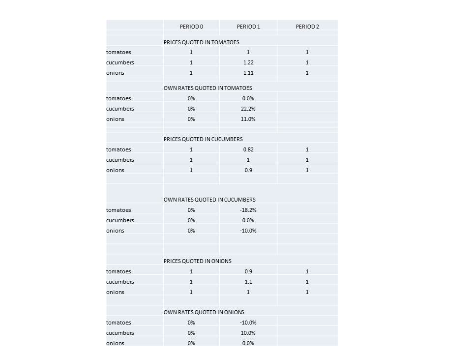
The table below shows prices and own rates for tomatoes, cucumbers and onions for each possible choice of numeraire. If prices are quoted in tomatoes, the price of tomatoes is fixed at 1. Given a zero real rate, the own rate on tomatoes in period is zero. What about the own rate on cucumbers? In period 0, with no change in prices expected, the own rate on cucumbers is also zero. However in period 1, after the price of cucumbers has risen to 1.22 tomatoes, the own rate on cucumbers must reflect the expected reduction in the price of a cucumber in terms of tomatoes from 1.22 tomatoes in period 1 to 1 tomato in period 2, a price reduction of 22% percent in terms of tomatoes, implying a cucumber own rate of 22% in terms of tomatoes. Similarly, the onion own rate in terms of tomatoes would be 11% percent reflecting a forward price for onions in terms of tomatoes 11% below the spot price for onions in terms of tomatoes. If prices were quoted in terms of cucumbers, the cucumber own rate would be zero, and because the prices of tomatoes and onions would be expected to rise in terms of cucumbers, the tomato and onion own rates would be negative (-18.2% for tomatoes and -10% for onions). And if prices were quoted in terms of onions, the onion own rate would be zero, while the tomato own rate, given the expected appreciation of tomatoes in terms of onions, would be negative (-10%), and the cucumber own rate, given the expected depreciation of cucumbers in terms of onions, would be positive (10%).

own_rates_in_terms_of_tomatoes_cucumbers_onions

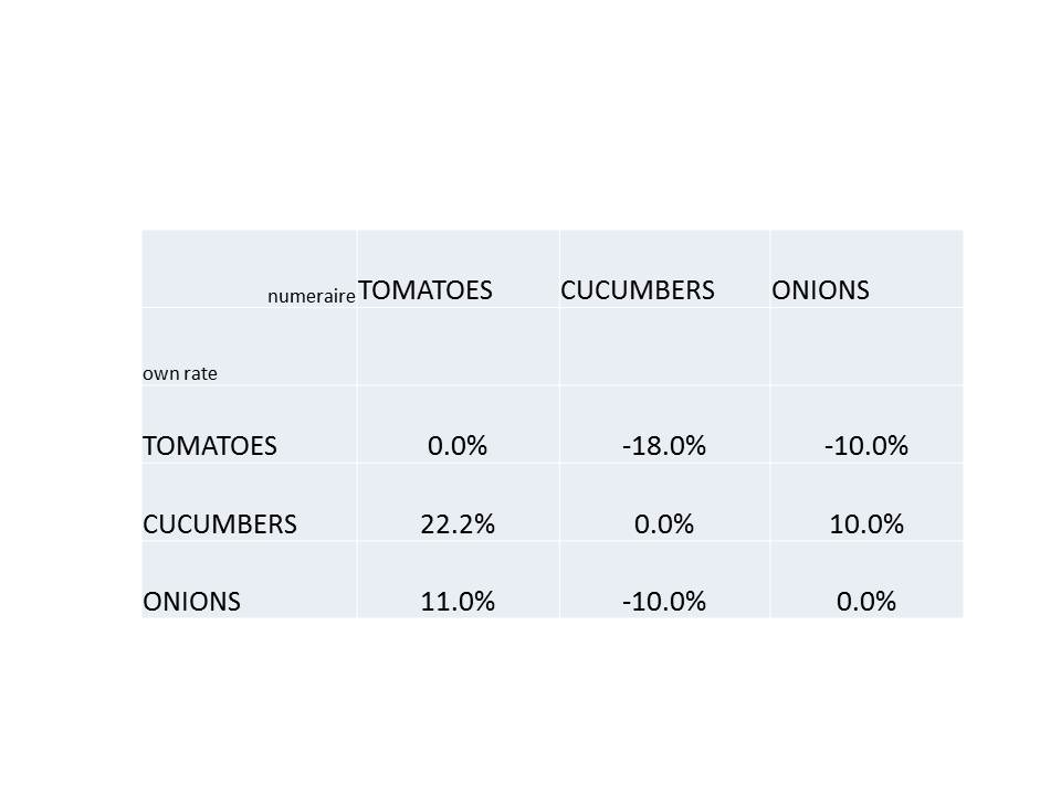
The next table, summarizing the first one, is a 3 by 3 matrix showing each of the nine possible combinations of numeraires and corresponding own rates.

own_rates_in_terms_of_tomatoes_cucumbers_onions_2

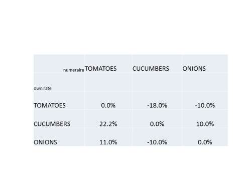
Thus, although the own rates of the different commodities differ, and although the commodity own rates differ depending on the choice of numeraire, the cost of borrowing (and the return to lending) is equal regardless of which commodity and which numeraire is chosen. As I stated in my previous post, Sraffa believed that, by showing that own rates can diverge, he showed that Hayek’s concept of a natural rate of interest was a nonsense notion. However, the differences in own rates, as Fisher had already showed 36 years earlier, are purely nominal. The underlying real rate, under Sraffa’s own analysis, is independent of the own rates.

Moreover, as I pointed out in my previous post, though the point was made in the context of a confused exposition of own rates,  whenever the own rate for a commodity is negative, there is an incentive to hold it now for sale in the next period at a higher price it would fetch in the current period. It is therefore only possible to observe negative own rates on commodities that are costly to store. Only if the cost of holding a commodity is greater than its expected appreciation would it not be profitable to withhold the commodity from sale this period and to sell instead in the following period. The rate of appreciation of a commodity cannot exceed the cost of storing it (as a percentage of its price).

What do I conclude from all this? That neither Sraffa nor Hayek adequately understood Fisher. Sraffa seems to have argued that there would be multiple real own rates of interest in disequilibrium — or at least his discussion of own rates seem to suggest that that is what he thought — while Hayek failed to see that there could be multiple nominal own rates. Fisher provided a definitive exposition of the distinction between real and nominal rates that encompasses both own rates and money rates of interest.

A. C. Pigou, the great and devoted student of Alfred Marshall, and ultimately his successor at Cambridge, is supposed to have said “It’s all in Marshall.” Well, one could also say “it’s all in Fisher.” Keynes, despite going out of his way in Chapter 12 of the General Theory to criticize Fisher’s distinction between the real and nominal rates of interest, actually vindicated Fisher’s distinction in his exposition of own rates in Chapter 17 of the GT, providing a valuable extension of Fisher’s analysis, but apparently failing to see the connection between his discussion and Fisher’s, and instead crediting Sraffa for introducing the own-rate analysis, even as he undermined Sraffa’s ambiguous suggestion that real own rates could differ. Go figure.

How to Think about Own Rates of Interest

Phil Pilkington has responded to my post about the latest version of my paper (co-authored by Paul Zimmerman) on the Sraffa-Hayek debate about the natural rate of interest. For those of you who haven’t been following my posts on the subject, here’s a quick review. Almost three years ago I wrote a post refuting Sraffa’s argument that Hayek’s concept of the natural rate of interest is incoherent, there being a multiplicity of own rates of interest in a barter economy (Hayek’s benchmark for the rate of interest undisturbed by monetary influences), which makes it impossible to identify any particular own rate as the natural rate of interest.

Sraffa maintained that if there are many own rates of interest in a barter economy, none of them having a claim to priority over the others, then Hayek had no basis for singling out any particular one of them as the natural rate and holding it up as the benchmark rate to guide monetary policy. I pointed out that Ludwig Lachmann had answered Sraffa’s attack (about 20 years too late) by explaining that even though there could be many own rates for individual commodities, all own rates are related by the condition that the cost of borrowing in terms of all commodities would be equalized, differences in own rates reflecting merely differences in expected appreciation or depreciation of the different commodities. Different own rates are simply different nominal rates; there is a unique real own rate, a point demonstrated by Irving Fisher in 1896 in Appreciation and Interest.

Let me pause here for a moment to explain what is meant by an own rate of interest. It is simply the name for the rate of interest corresponding to a loan contracted in terms of a particular commodity, the borrower receiving the commodity now and repaying the lender with the same commodity when the term of the loan expires. Sraffa correctly noted that in equilibrium arbitrage would force the terms of such a loan (i.e., the own rate of interest) to equal the ratio of the current forward price of the commodity to its current spot price, buying spot and selling forward being essentially equivalent to borrowing and repaying.

Now what is tricky about Sraffa’s argument against Hayek is that he actually acknowledges at the beginning of his argument that in a stationary equilibrium, presumably meaning that prices remain at their current equilibrium levels over time, all own rates would be equal. In fact if prices remain (and are expected to remain) constant period after period, the ratio of forward to spot prices would equal unity for all commodities implying that the natural rate of interest would be zero. Sraffa did not make that point explicitly, but it seems to be a necessary implication of his analysis. (This implication seems to bear on an old controversy in the theory of capital and interest, which is whether the rate of interest would be positive in a stationary equilibrium with constant real income). Schumpeter argued that the equilibrium rate of interest would be zero, and von Mises argued that it would be positive, because time preference implying that the rate of interest is necessarily always positive is a kind of a priori praxeological law of nature, the sort of apodictic gibberish to which von Mises was regrettably predisposed. The own-rate analysis supports Schumpeter against Mises.

So to make the case against Hayek, Sraffa had to posit a change, a shift in demand from one product to another, that disrupts the pre-existing equilibrium. Here is the key passage from Sraffa:

Suppose there is a change in the distribution of demand between various commodities; immediately some will rise in price, and others will fall; the market will expect that, after a certain time, the supply of the former will increase, and the supply of the latter fall, and accordingly the forward price, for the date on which equilibrium is expected to be restored, will be below the spot price in the case of the former and above it in the case of the latter; in other words, the rate of interest on the former will be higher than on the latter. (p. 50)

This is a difficult passage, and in previous posts, and in my paper with Zimmerman, I did not try to parse this passage. But I am going to parse it now. Assume that demand shifts from tomatoes to cucumbers. In the original equilibrium, let the prices of both be $1 a pound. With a zero own rate of interest in terms of both tomatoes and cucumbers, you could borrow a pound of tomatoes today and discharge your debt by repaying the lender a pound of tomatoes at the expiration of the loan. However, after the demand shift, the price of tomatoes falls to, say, $0.90 a pound, and the price of cucumbers rises to, say, $1.10 a pound. Sraffa posits that the price changes are temporary, not because the demand shift is temporary, but because the supply curves of tomatoes and cucumbers are perfectly elastic at $1 a pound. However, supply does not adjust immediately, so Sraffa believes that there can be a temporary deviation from the long-run equilibrium prices of tomatoes and cucumbers.

The ratio of the forward prices to the spot prices tells you what the own rates are for tomatoes and cucumbers. For tomatoes, the ratio is 1/.9, implying an own rate of 11.1%. For cucumbers the ratio is 1/1.1, implying an own rate of -9.1%. Other prices have not changed, so all other own rates remain at 0. Having shown that own rates can diverge, Sraffa thinks that he has proven Hayek’s concept of a natural rate of interest to be a nonsense notion. He was mistaken.

There are at least two mistakes. First, the negative own rate on cucumbers simply means that no one will lend in terms of cucumbers for negative interest when other commodities allow lending at zero interest. It also means that no one will hold cucumbers in this period to sell at a lower price in the next period than the cucumbers would fetch in the current period. Cucumbers are a bad investment, promising a negative return; any lending and investing will be conducted in terms of some other commodity. The negative own rate on cucumbers signifies a kind of corner solution, reflecting the impossibility of transporting next period’s cucumbers into the present. If that were possible cucumber prices would be equal in the present and the future, and the cucumber own rate would be equal to all other own rates at zero. But the point is that if any lending takes place, it will be at a zero own rate.

Second, the positive own rate on tomatoes means that there is an incentive to lend in terms of tomatoes rather than lend in terms of other commodities. But as long as it is possible to borrow in terms of other commodities at a zero own rate, no one borrows in terms of tomatoes. Thus, if anyone wanted to lend in terms of tomatoes, he would have to reduce the rate on tomatoes to make borrowers indifferent between borrowing in terms of tomatoes and borrowing in terms of some other commodity. However, if tomatoes today can be held at zero cost to be sold at the higher price prevailing next period, currently produced tomatoes would be sold in the next period rather than sold today. So if there were no costs of holding tomatoes until the next period, the price of tomatoes in the next period would be no higher than the price in the current period. In other words, the forward price of tomatoes cannot exceed the current spot price by more than the cost of holding tomatoes until the next period. If the difference between the spot and the forward price reflects no more than the cost of holding tomatoes till the next period, then, as Keynes showed in chapter 17 of the General Theory, the own rates are indeed effectively equalized after appropriate adjustment for storage costs and expected appreciation.

Thus, it was Keynes, who having selected Sraffa to review Hayek’s Prices and Production in the Economic Journal, of which Keynes was then the editor, adapted Sraffa’s own rate analysis in the General Theory, but did so in a fashion that, at least partially, rehabilitated the very natural-rate analysis that had been the object of Sraffa’s scorn in his review of Prices and Production. Keynes also rejected the natural-rate analysis, but he did so not because it is nonsensical, but because the natural rate is not independent of the level of employment. Keynes’s argument that the natural rate depends on the level of employment seems to me to be inconsistent with the idea that the IS curve is downward sloping. But I will have to think about that a bit and reread the relevant passage in the General Theory and perhaps revisit the point in a future post.

 UPDATE (07/28/14 13:02 EDT): Thanks to my commenters for pointing out that my own thinking about the own rate of interest was not quite right. I should have defined the own rate in terms of a real numeraire instead of $, which was a bit of awkwardness that I should have fixed before posting. I will try to publish a corrected version of this post later today or tomorrow. Sorry for posting without sufficient review and revision.

UPDATE (08/04/14 11:38 EDT): I hope to post the long-delayed sequel to this post later today. A number of personal issues took precedence over posting, but I also found it difficult to get clear on several minor points, which I hope that I have now resolved adequately, for example I found that defining the own rate in terms of a real numeraire was not really the source of my problem with this post, though it was a useful exercise to work through. Anyway, stay tuned.

A New Version of my Paper (with Paul Zimmerman) on the Hayek-Sraffa Debate Is Available on SSRN

One of the good things about having a blog (which I launched July 5, 2011) is that I get comments about what I am writing about from a lot of people that I don’t know. One of my most popular posts – it’s about the sixteenth most visited — was one I wrote, just a couple of months after starting the blog, about the Hayek-Sraffa debate on the natural rate of interest. Unlike many popular posts, to which visitors are initially drawn from very popular blogs that linked to those posts, but don’t continue to drawing a lot of visitors, this post initially had only modest popularity, but still keeps on drawing visitors.

That post also led to a collaboration between me and my FTC colleague Paul Zimmerman on a paper “The Sraffa-Hayek Debate on the Natural Rate of Interest” which I presented two years ago at the History of Economics Society conference. We have now finished our revisions of the version we wrote for the conference, and I have just posted the new version on SSRN and will be submitting it for publication later this week.

Here’s the abstract posted on the SSRN site:

Hayek’s Prices and Production, based on his hugely successful lectures at LSE in 1931, was the first English presentation of Austrian business-cycle theory, and established Hayek as a leading business-cycle theorist. Sraffa’s 1932 review of Prices and Production seems to have been instrumental in turning opinion against Hayek and the Austrian theory. A key element of Sraffa’s attack was that Hayek’s idea of a natural rate of interest, reflecting underlying real relationships, undisturbed by monetary factors, was, even from Hayek’s own perspective, incoherent, because, without money, there is a multiplicity of own rates, none of which can be uniquely identified as the natural rate of interest. Although Hayek’s response failed to counter Sraffa’s argument, Ludwig Lachmann later observed that Keynes’s treatment of own rates in Chapter 17 of the General Theory (itself a generalization of Fisher’s (1896) distinction between the real and nominal rates of interest) undercut Sraffa’s criticism. Own rates, Keynes showed, cannot deviate from each other by more than expected price appreciation plus the cost of storage and the commodity service flow, so that anticipated asset yields are equalized in intertemporal equilibrium. Thus, on Keynes’s analysis in the General Theory, the natural rate of interest is indeed well-defined. However, Keynes’s revision of Sraffa’s own-rate analysis provides only a partial rehabilitation of Hayek’s natural rate. There being no unique price level or rate of inflation in a barter system, no unique money natural rate of interest can be specified. Hayek implicitly was reasoning in terms of a constant nominal value of GDP, but barter relationships cannot identify any path for nominal GDP, let alone a constant one, as uniquely compatible with intertemporal equilibrium.

Aside from clarifying the conceptual basis of the natural-rate analysis and its relationship to Sraffa’s own-rate analysis, the paper also highlights the connection (usually overlooked but mentioned by Harald Hagemann in his 2008 article on the own rate of interest for the International Encyclopedia of the Social Sciences) between the own-rate analysis, in either its Sraffian or Keynesian versions, and Fisher’s early distinction between the real and nominal rates of interest. The conceptual identity between Fisher’s real and nominal distinction and Keynes’s own-rate analysis in the General Theory only magnifies the mystery associated with Keynes’s attack in chapter 13 of the General Theory on Fisher’s distinction between the real and the nominal rates of interest.

I also feel that the following discussion of Hayek’s role in developing the concept of intertemporal equilibrium, though tangential to the main topic of the paper, makes an important point about how to think about intertemporal equilibrium.

Perhaps the key analytical concept developed by Hayek in his early work on monetary theory and business cycles was the idea of an intertemporal equilibrium. Before Hayek, the idea of equilibrium had been reserved for a static, unchanging, state in which economic agents continue doing what they have been doing. Equilibrium is the end state in which all adjustments to a set of initial conditions have been fully worked out. Hayek attempted to generalize this narrow equilibrium concept to make it applicable to the study of economic fluctuations – business cycles – in which he was engaged. Hayek chose to formulate a generalized equilibrium concept. He did not do so, as many have done, by simply adding a steady-state rate of growth to factor supplies and technology. Nor did Hayek define equilibrium in terms of any objective or measurable magnitudes. Rather, Hayek defined equilibrium as the mutual consistency of the independent plans of individual economic agents.

The potential consistency of such plans may be conceived of even if economic magnitudes do not remain constant or grow at a constant rate. Even if the magnitudes fluctuate, equilibrium is conceivable if the fluctuations are correctly foreseen. Correct foresight is not the same as perfect foresight. Perfect foresight is necessarily correct; correct foresight is only contingently correct. All that is necessary for equilibrium is that fluctuations (as reflected in future prices) be foreseen. It is not even necessary, as Hayek (1937) pointed out, that future price changes be foreseen correctly, provided that individual agents agree in their anticipations of future prices. If all agents agree in their expectations of future prices, then the individual plans formulated on the basis of those anticipations are, at least momentarily, equilibrium plans, conditional on the realization of those expectations, because the realization of those expectations would allow the plans formulated on the basis of those expectations to be executed without need for revision. What is required for intertemporal equilibrium is therefore a contingently correct anticipation by future agents of future prices, a contingent anticipation not the result of perfect foresight, but of contingently, even fortuitously, correct foresight. The seminal statement of this concept was given by Hayek in his classic 1937 paper, and the idea was restated by J. R. Hicks (1939), with no mention of Hayek, two years later in Value and Capital.

I made the following comment in a footnote to the penultimate sentence of the quotation:

By defining correct foresight as a contingent outcome rather than as an essential property of economic agents, Hayek elegantly avoided the problems that confounded Oskar Morgenstern ([1935] 1976) in his discussion of the meaning of equilibrium.

I look forward to reading your comments.

Does Macroeconomics Need Financial Foundations?

One of the little instances of collateral damage occasioned by the hue and cry following upon Stephen Williamson’s post arguing that quantitative easing has been deflationary was the dustup between Scott Sumner and financial journalist and blogger Izabella Kaminska. I am not going to comment on the specifics of their exchange except to say that the misunderstanding and hard feelings between them seem to have been resolved more or less amicably. However, in quickly skimming the exchange between them, I was rather struck by the condescending tone of Kaminska’s (perhaps understandable coming from the aggrieved party) comment about the lack of comprehension by Scott and Market Monetarists more generally of the basics of finance.

First I’d just like to say I feel much of the misunderstanding comes from the fact that market monetarists tend to ignore the influence of shadow banking and market plumbing in the monetary world. I also think (especially from my conversation with Lars Christensen) that they ignore technological disruption, and the influence this has on wealth distribution and purchasing decisions amongst the wealthy, banks and corporates. Also, as I outlined in the post, my view is slightly different to Williamson’s, it’s based mostly on the scarcity of safe assets and how this can magnify hoarding instincts and fragment store-of-value markets, in a Gresham’s law kind of way. Expectations obviously factor into it, and I think Williamson is absolutely right on that front. But personally I don’t think it’s anything to do with temporary or permanent money expansion expectations. IMO It’s much more about risk expectations, which can — if momentum builds — shift very very quickly, making something deflationary, inflationary very quickly. Though, that doesn’t mean I am worried about inflation (largely because I suspect we may have reached an important productivity inflection point).

This remark was followed up with several comments blasting Market Monetarists for their ignorance of the basics of finance and commending Kaminska for the depth of her understanding to which Kaminska warmly responded adding a few additional jibes at Sumner and Market Monetarists. Here is one.

Market monetarists are getting testy because now that everybody started scrutinizing QE they will be exposed as ignorant. The mechanisms they originally advocated QE would work through will be seen as hopelessly naive. For them the money is like glass beads squirting out of the Federal Reserve, you start talking about stuff like collateral, liquid assets, balance sheets and shadow banking and they are out of their depth.

For laughs: Sumner once tried to defend the childish textbook model of banks lending out reserves and it ended in a colossal embarrassment in the comments section http://www.themoneyillusion.com/?p=5893

For you to defend your credentials in front of such “experts” is absurd. There is a lot more depth to your understanding than to their sandbox vision of the monetary system. And yes, it *is* crazy that journalists and bloggers can talk about these things with more sense than academics. But this [is] the world we live in.

To which Kaminska graciously replied:

Thanks as well! And I tend to agree with your assessment of the market monetarist view of the world.

So what is the Market Monetarist view of the world of which Kaminska tends to have such a low opinion? Well, from reading Kaminska’s comments and those of her commenters, it seems to be that Market Monetarists have an insufficiently detailed and inaccurate view of financial intermediaries, especially of banks and shadow banks, and that Market Monetarists don’t properly understand the role of safe assets and collateral in the economy. But the question is why, and how, does any of this matter to a useful description of how the economy works?

Well, this whole episode started when Stephen Williamson had a blog post arguing that QE was deflationary, and the reason it’s deflationary is that creating more high powered money provides the economy with more safe assets and thereby reduces the liquidity premium associated with safe assets like short-term Treasuries and cash. By reducing the liquidity premium, QE causes the real interest rate to fall, which implies a lower rate of inflation.

Kaminska thinks that this argument, which Market Monetarists find hard to digest, makes sense, though she can’t quite bring herself to endorse it either. But she finds the emphasis on collateral and safety and market plumbing very much to her taste. In my previous post, I raised what I thought were some problems with Williamson’s argument.

First, what is the actual evidence that there is a substantial liquidity premium on short-term Treasuries? If I compare the rates on short-term Treasuries with the rates on commercial paper issued by non-Financial institutions, I don’t find much difference. If there is a substantial unmet demand for good collateral, and there is only a small difference in yield between commercial paper and short-term Treasuries, one would think that non-financial firms could make a killing by issuing a lot more commercial paper. When I wrote the post, I was wondering whether I, a financial novice, might be misreading the data or mismeasuring the liquidity premium on short-term Treasuries. So far, no one has said anything about that, but If I am wrong, I am happy to be enlightened.

Here’s something else I don’t get. What’s so special about so-called safe assets? Suppose, as Williamson claims, that there’s a shortage of safe assets. Why does that imply a liquidity premium? One could still compensate for the lack of safety by over-collateralizing the loan using an inferior asset. If that is a possibility, why is the size of the liquidity premium not constrained?

I also pointed out in my previous post that a declining liquidity premium would be associated with a shift out of money and into real assets, which would cause an increase in asset prices. An increase in asset prices would tend to be associated with an increase in the value of the underlying service flows embodied in the assets, in other words in an increase in current prices, so that, if Williamson is right, QE should have caused measured inflation to rise even as it caused inflation expectations to fall. Of course Williamson believes that the decrease in liquidity premium is associated with a decline in real interest rates, but it is not clear that a decline in real interest rates has any implications for the current price level. So Williamson’s claim that his model explains the decline in observed inflation since QE was instituted does not seem all that compelling.

Now, as one who has written a bit about banking and shadow banking, and as one who shares the low opinion of the above-mentioned commenter on Kaminska’s blog about the textbook model (which Sumner does not defend, by the way) of the money supply via a “money multiplier,” I am in favor of changing how the money supply is incorporated into macromodels. Nevertheless, it is far from clear that changing the way that the money supply is modeled would significantly change any important policy implications of Market Monetarism. Perhaps it would, but if so, that is a proposition to be proved (or at least argued), not a self-evident truth to be asserted.

I don’t say that finance and banking are not important. Current spreads between borrowing and lending rates, may not provide a sufficient margin for banks to provide the intermediation services that they once provided to a wide range of customers. Businesses have a wider range of options in obtaining financing than they used to, so instead of holding bank accounts with banks and foregoing interest on deposits to be able to have a credit line with their banker, they park their money with a money market fund and obtain financing by issuing commercial paper. This works well for firms large enough to have direct access to lenders, but smaller businesses can’t borrow directly from the market and can only borrow from banks at much higher rates or by absorbing higher costs on their bank accounts than they would bear on a money market fund.

At any rate, when market interest rates are low, and when perceived credit risks are high, there is very little margin for banks to earn a profit from intermediation. If so, the money multiplier — a crude measure of how much intermediation banks are engaging in goes down — it is up to the monetary authority to provide the public with the liquidity they demand by increasing the amount of bank reserves available to the banking system. Otherwise, total spending would contract sharply as the public tried to build up their cash balances by reducing their own spending – not a pretty picture.

So finance is certainly important, and I really ought to know more about market plumbing and counterparty risk  and all that than I do, but the most important thing to know about finance is that the financial system tends to break down when the jointly held expectations of borrowers and lenders that the loans that they agreed to would be repaid on schedule by the borrowers are disappointed. There are all kinds of reasons why, in a given case, those jointly held expectations might be disappointed. But financial crises are associated with a very large cluster of disappointed expectations, and try as they might, the finance guys have not provided a better explanation for that clustering of disappointed expectations than a sharp decline in aggregate demand. That’s what happened in the Great Depression, as Ralph Hawtrey and Gustav Cassel and Irving Fisher and Maynard Keynes understood, and that’s what happened in the Little Depression, as Market Monetarists, especially Scott Sumner, understand. Everything else is just commentary.

Hawtrey’s Good and Bad Trade: Part II

Here I am again back at you finally with another installment in my series on Hawtrey’s Good and Bad Trade. In my first installment I provided some background on Hawtrey and a quick overview of the book, including a mention of the interesting fact (brought to my attention by David Laidler) that Hawtrey used the term “effective demand” in pretty much the same way that Keynes, some 20 years later, would use it in the General Theory.

In this post, I want to discuss what I consider the highlights of the first six chapters. The first chapter is a general introduction to the entire volume laying out the basic premise of the book, which is that the business cycle, understood as recurring fluctuations in the level of employment, is the result of monetary disturbances that lead to alternating phases of expansion and contraction. It is relatively easy for workers to find employment in expansions, but more difficult to do so in contractions. From the standpoint of the theory of economic equilibrium, the close correlation between employment and nominal income over the business cycle is somewhat paradoxical, because, according to the equilibrium theory, the allocation of resources is governed by relative, not absolute, prices. In the theory of equilibrium, a proportional increase or decrease in all prices should have no effect on employment. To explain the paradox, Hawtrey relies on the rigidity of some prices, and especially wages, an empirical fact that, Hawtrey believed, was an essential aspect of any economic system, and a necessary condition for the cyclicality of output and employment.

In Hawtrey’s view, economic expansions and contractions are caused by variations in effective demand, which he defines as total money income. (For reasons I discussed about a year and a half ago, I prefer to define “effective demand” as total money expenditure.) What determines effective demand, according to Hawtrey, is the relationship between the amount of money people are holding and the amount that they would, on average over time, like to hold. The way to think about the amount of money that people would like to hold is to imagine that there is some proportion of their annual income that people aim to hold in the form of cash.

The relationship between the amount of cash being held and the amount that people would like to hold depends on the nature of the monetary system. Hawtrey considers two types of monetary system: one type (discussed in chapter 2) is a pure fiat money system in which all money is issued by government; the other (discussed in chapter 3) is a credit system in which money is also created by banks by promising to redeem, on demand, their obligations (either deposits or negotiable banknotes) for fiat money. Credit money is issued by banks in exchange for a variety of assets, usually the untraded IOUs of borrowers.

In a pure fiat money system, effective demand depends chiefly on the amount of fiat money that people want to hold and on the amount of fiat money created by the government, fiat money being the only money available. A pure fiat money system, Hawtrey understood, was just the sort of system in which the propositions of the quantity theory of money would obtain at least in the medium to long run.

[I]f the adjustment [to a reduction in the quantity of money] could be made entirely by a suitable diminution of wages and salaries, accompanied by a corresponding diminution of prices, the commercial community could be placed forthwith in a new position of equilibrium, in which the output would continue unchanged, and distribution would only be modified by the apportionment of a somewhat larger share of the national product to the possessors of interest, rent, and other kinds of fixed incomes. In fact, the change in the circulating medium is merely a change in the machinery of distribution, and a change, moreover, which, once made, does not impair the effectiveness of that machinery. If the habits of the community are adapted without delay to the change, the production of wealth will continue unabated. If customary prices resist the change, the adjustment, which is bound to come sooner or later, will only be forced upon the people by the pressure of distress. (p. 41)

In a fiat money system, if the public have less money than they would like to hold their only recourse is to attempt to reduce their expenditures relative to their receipts, either offering more in exchange, which tends to depress prices or reducing their purchases, making it that much more difficult for anyone to increase sales except by reducing prices. The problem is that in a fiat system the amount of money is what it is, so that if one person manages to increase his holdings of money by increasing sales relative to purchases, his increase in cash balances must have be gained at the expense of someone else. With a fixed amount of fiat money in existence, the public as a whole cannot increase their holdings of cash, so equilibrium can be restored only by reducing the quantity of money demanded. But the reduction in the amount of money that people want to hold cannot occur unless income in money terms goes down. Money income can go down only if total output in real terms, or if the price level, falls. With nominal income down, people, wanting to hold some particular share of their nominal income in the form of money, will be content with a smaller cash balance than they were before, and will stop trying to increase their cash balances by cutting their expenditure. Because some prices — and especially wages — tend to be sticky, Hawtrey felt that it was inevitable that the adjustment to reduction in the amount of fiat money would cause both real income and prices to fall.

Although Hawtrey correctly perceived that the simple quantity theory would not, even in theory, hold precisely for a credit system, his analysis of the credit system was incomplete inasmuch as he did not fully take into account the factors governing the public’s choice between holding credit money as opposed to fiat money or the incentives of the banking system to create credit money. That theory was not worked out till James Tobin did so 50 years later (another important anniversary worthy of note), though John Fullarton made an impressive start in his great work on the subject in 1844, a work Hawtrey must have been familiar with, but, to my knowledge, never discussed in detail.

In such a banking system there is no necessary connexion between the total of the deposits and the amount of coin which has been paid to the banks. A banker may at any time grant a customer a loan by simply adding to the balance standing to the customer’s credit in the books of the bank. No cash passes, but the customer acquires the right, during the currency of the loan, to draw cheques on the bank up to the amount lent. When the period of the loan expires, if the customer has a large enough balance to his credit, the loan can be repaid without any cash being employed, the amount of the loan being simply deducted from the balance. So long as the loan is outstanding it represents a clear addition to the available stock of “money,” in the sense of purchasing power. It is “money” in the the sense which will play, in a community possessing banks, the same part as money in the stricter sense of legal tender currency would play in the fictitious bankless community whose commercial conditions we previously have been considering. This is the most distinctive feature of the banking system, that between the stock of legal tender currency and the trading community there is interposed an intermediary, the banker, who can, if he wishes, create money out of nothing. (PP. 56-57)

This formulation is incomplete, inasmuch as it leaves the decision of the banker about how much money to create unconstrained by the usual forces of marginal revenue and marginal cost that supposedly determine the decisions of other profit-seeking businessmen. Hawtrey is not oblivious to the problem, but does not advance the analysis as far as he might have.

We have now to find out how this functionary uses his power and under what limitations he works. Something has already been said of the contingencies for which he must provide. Whenever he grants a loan and thereby creates money, he must expect a certain portion of this money to be applied sooner or later, to purposes for which legal tender currency is necessary. Sums will be drawn out from time to time to be spent either in wages or in small purchases, and the currency so applied will take a little time to find its way back to the banks. Large purchases will be paid for by cheque, involving a mere transfer of credit from one banking account to another, but the recipient of the cheque may wish to apply it ot the payment of wages, etc. Thus the principal limitation upon the banker’s freedom to create money is that he must have a reserve to meet the fresh demands for cash to which the creation of new money may lead. (Id.)

This is a very narrow view, apparently assuming that there is but one banker and that the only drain on the reserves of the banker is the withdrawal of currency by depositors. The possibility that recipients of cheques drawn on one bank may prefer to hold those funds in a different bank so that the bank must pay a competitive rate of interest on its deposits to induce its deposits to be held rather than those of another bank is not considered.

In trade a seller encourages or discourages buyers by lowering or raising his prices. So a banker encourages or discourages borrowers by lowering or raising the rate of interest. (p.58)

Again, Hawtrey only saw half the picture. The banker is setting two rates: the rate that he charges borrowers and the rate that he pays to depositors. It is the spread between those two rates that determines the marginal revenue from creating another dollar of deposits. Given that marginal revenue, the banker must form some estimate of the likely cost associated with creating another dollar of deposits (an estimate that depends to a large degree on expectations that may or may not be turn out to be correct), and it is the comparison between the marginal revenue from creating additional deposits with the expected cost of creating additional deposits that determines whether a bank wants to expand or contract its deposits.

Of course, the incomplete analysis of the decision making of the banker is not just Hawtrey’s, it is characteristic of all Wicksellian natural-rate theories. However, in contrast to other versions of the natural-rate genre, Hawtrey managed to avoid the logical gap in those theories: the failure to see that it is the spread between the lending and the deposit rates, not the difference between the lending rate and the natural rate, that determines whether banks are trying to expand or contract. But that is a point that I will have to come back to in the next installment in this series in which I will try to follow through the main steps of Hawtrey’s argument about how a banking system adjusts to a reduction in the quantity of fiat money (aka legal tender currency or base money) is reduced. That analysis, which hinges on the role of merchants and traders whose holding of inventories of goods is financed by borrowing from the banks, was a critical intellectual innovation of Hawtrey’s and was the key to his avoidance of the Wicksellian explanatory gap.

Hicks on Keynes and the Theory of the Demand for Money

One of my favorite papers is one published by J. R. Hicks in 1935 “A Suggestion for Simplifying the Demand for Theory of Money.” The aim of that paper was to explain how to reconcile the concept of a demand for money into the theory of rational choice. Although Marshall had attempted to do so in his writings, his formulations of the idea were not fully satisfactory, and other Cambridge economists, notably Pigou, Lavington, Robertson, and Keynes, struggled to express the idea in a more satisfactory way than Marshall had done.

In Hicks’s introductory essay to volume II of his Collected Essays on Economic Theory in which his 1935 essay appears, Hicks recounts that Keynes told him after reading his essay that the essay was similar to the theory of liquidity preference, on which Keynes was then working.

To anyone who comes over from the theory of value to the theory of money, there are a number of things which are rather startling. Chief of these is the preoccupation of monetary theorists with a certain equation, which states that the price of goods multiplied by the quantity of goods equals the amount of money which is spent on them. The equation crops up again and again, and it has all sorts of ingenious little arithmetical tricks performed on it. Sometimes it comes out as MV = PT . . .

Now we, of the theory of value, are not unfamiliar with this equation, and there was a time when we used to attach as much importance to it as monetary theorists seem to do still. This was in the middle of the last century, when we used to talk about value being “a ratio between demand and supply.” Even now, we accept the equation, and work it, more or less implicitly, into our systems. But we are rather inclined to take it for granted, since it is rather tautologous, and since we have found that another equation, not alternative to the quantity equation, but complementary with it, is much more significant. This is the equation which states that the relative value of two commodities depends upon their relative marginal utility.

Now to an ingénue, who comes over to monetary theory, it is extremely trying to be deprived of this sheet-anchor. It was marginal utility that really made sense of the theory of value; and to come to a branch of economics which does without marginal utility altogether! No wonder there are such difficulties and such differences! What is wanted is a “marginal revolution!”

That is my suggestion. But I know that it will meet with apparently crushing objections. I shall be told that the suggestion has been tried out before. It was tried by Wicksell, and though it led to interesting results, it did not lead to a marginal utility theory of money. It was tried by Mises, and led to the conclusion that money is a ghost of gold – because, so it appeared, money as such has no marginal utility. The suggestion has a history, and its history is not encouraging.

This would be enough to frighten one off, were it not for two things. Both in the theory of value and in the theory of money there have been developments in the twenty of thirty years since Wicksell and Mises wrote. And these developments have considerably reduced the barriers that blocked their way.

In the theory of value, the work of Pareto, Wicksteed, and their successors, has broadened and deepened our whole conception of marginal utility. We now realize that the marginal utility analysis is nothing else than a general theory of choice, which is applicable whenever the choice is between alternatives that are capable of quantitative expression. Now money is obviously capable of quantitative expression, and therefore the objection that money has no marginal utility must be wrong. People do choose to have money rather than other things, and therefore, in the relevant sense, money must have a marginal utility.

But merely to call their marginal utility X, and then proceed to draw curves, would not be very helpful. Fortunately the developments in monetary theory to which I alluded come to our rescue.

Mr. Keynes’s Treatise, so far as I have been able to discover, contains at least three theories of money. One of them is the Savings and Investment theory, which . . . seems to me only a quantity theory much glorified. One of them is a Wicksellian natural rate theory. But the third is altogether more interesting. It emerges when Mr. Keynes begins to talk about the price-level of investment goods; when he shows that this price-level depends upon the relative preference of the investor – to hold bank-deposits or to hold securities. Here at last we have something which to a value theorist looks sensible and interesting! Here at last we have a choice at the margin! And Mr. Keynes goes on to put substance into our X, by his doctrine that the relative preference depends upon the “bearishness” or “bullishness” of the public, upon their relative desire for liquidity or profit.

My suggestion may, therefore, be reformulated. It seems to me that this third theory of Mr. Keynes really contains the most important of his theoretical contribution; that here, at last, we have something which, on the analogy (the approximate analogy) of value theory, does begin to offer a chance of making the whole thing easily intelligible; that it si form this point, not from velocity of circulation, or Saving and Investment, that we ought to start in constructing the theory of money. But in saying this I am being more Keynesian than Keynes [note to Blue Aurora this was written in 1934 and published in 1935].

The point of this extended quotation, in case it is not obvious to the reader, is that Hicks is here crediting Keynes in his Treatise on Money with a crucial conceptual advance in formulating a theory of the demand for money consistent with the marginalist theory of value. Hicks himself recognized that Keynes in the General Theory worked out a more comprehensive version of the theory than that which he presented in his essay, even though they were not entirely the same. So there was no excuse for Friedman to present a theory of the demand for money which he described “as part of capital or wealth theory, concerned with the composition of the balance sheet or portfolio of assets,” without crediting Keynes for that theory, just because he rejected the idea of absolute liquidity preference.

Here is how Hicks summed up the relationship in his introductory essay referred to above.

Keynes’s Liquidity theory was so near to mine, and was put over in so much more effective a way than I could hope to achieve, that it seemed pointless, at first, to emphasize differences. Sometimes, indeed, he put his in such a way that there was hardly any difference. But, as time went on, what came to be regarded in many quarters, as Keynesian theory was something much more mechanical than he had probably intended. It was certainly more mechanical than I had intended. So in the end I had ot go back to “Simplifying,” and to insist that its message was a Declaration of Independence, not only from the “free market” school from which I was expressly liberating myself, but also from what came to pass as Keynesian economics.

Liquidity Trap or Credit Deadlock

In earlier posts in my series about Hawtrey and Keynes, I’ve mentioned the close connection between Hawtrey’s concept of a “credit deadlock” and the better-known Keynesian concept of a “liquidity trap,” a term actually coined by J. R. Hicks in his classic paper summarizing the Keynesian system by way of the IS-LM model. As I’ve previously noted, the two concepts, though similar, are not identical, a characteristic of much of their work on money and business cycles. Their ideas, often very similar, almost always differ in some important way, often leading to sharply different policy implications. Keynes recognized the similarities in their thinking, acknowledging his intellectual debt to Hawtrey several times, but, on occasion, Keynes could not contain his frustration and exasperation with what he felt was Hawtrey’s obstinate refusal to see what he was driving at.

In this post, commenter GDF asked me about the credit deadlock and the liquidity trap:

Would you mind explaining your thoughts apropos of differences between Hawtrey’s credit deadlock theory and Keynes’ liquidity trap. It seems to me that modern liquidity trapists like Krugman, Woodford etc. have more in common with Hawtrey than Keynes in the sense that they deal with low money demand elasticity w.r.t. the short rate rather than high money demand elasticity w.r.t. the long rate.

To which I answered:

My view is that credit deadlock refers to a situation of extreme entrepreneurial pessimism, which I would associate with negative real rates of interest. Keynes’s liquidity trap occurs at positive real rates of interest (not the zero lower bound) because bear bond speculators will not allow the long-term rate to fall below some lower threshold because of the risk of suffering a capital loss on long-term bonds once the interest rate rises. Hawtrey did not think much of this argument.

Subsequently in this post, commenter Rob Rawlings suggested that I write about the credit deadlock and provided a link to a draft of a paper by Roger Sandilands, “Hawtreyan ‘Credit Deadlock’ or Keynesian ‘Liquidity Trap’? Lessons for Japan from the Great Depression” (eventually published as the final chapter in the volume David Laidler’s Contributions to Economics, edited by Robert Leeson, an outstanding collection of papers celebrating one of the greatest economists of our time). In our recent exchange of emails about Hawtrey, Laidler also drew my attention to Sandilands’s paper.

Sandilands’s paper covers an extremely wide range of topics in both the history of economics (mainly about Hawtrey and especially the largely forgotten Laughlin Currie), the history of the Great Depression, and the chronic Japanese deflation and slowdown since the early 1990s. But for this post, the relevant point from Sandilands’s paper is the lengthy quotation with which he concludes from Laidler’s paper, “Woodford and Wicksell on Interest and Prices: The Place of the Pure Credit Economy in the Theory of Monetary Policy.”

To begin with, a “liquidity trap” is a state of affairs in which the demnd for money becomes perfectly elastic with respect to a long rate of interest at some low positive level of the latter. Until the policy of “quantitative easing” was begun in 2001, the ratio of the Japanese money stock to national income, whether money was measured by the base, M1, or any broader aggregate, rose slowly at best, and it was short, not long, rates of interest that were essentially zero. Given these facts, it is hard to see what the empirical basis for the diagnosis of a liquidity trap could have been. On the other hand, and again before 2001, the empirical evidence gave no reason to reject the hypothesis that a quite separate and distinct phenomenon was at work, namely a Hawtreyan “credit deadlock”. Here the problem is not a high elasticity of the economy’s demand for money with respect to the long rate of interest, but a low elasticity of its demand for bank credit with respect to the short rate, which inhibits the borrowing that is a necessary prerequisite for money creation. The solution to a credit deadlock, as Hawtrey pointed out, is vigorous open market operations to bring about increases in the monetary base, and therefore the supply of chequable deposits, that mere manipulation of short term interest rates is usually sufficient to accomplish in less depressed times.

Now the conditions for a liquidity trap might indeed have existed in Japan in the 1990s. Until the credit deadlock affecting its monetary system was broken by quantitative easing in 2001 . . . it was impossible to know this. As it has happened, however, the subsequent vigorous up-turn of the Japanese economy that began in 2002 and is still proceeding is beginning to suggest that there was no liquidity trap at work in that economy. If further evidence bears out this conclusion, a serious policy error was made in the 1990s, and that error was based on a theory of monetary policy that treats the short interest rate as the central bank’s only tool, and characterizes the transmission mechanism as working solely through the influence of interest rates on aggregate demand.

That theory provided no means for Japanese policy makers to distinguish between a liquidity trap, which is a possible feature of the demand for money function, and a credit deadlock which is a characteristic of the money supply process, or for them to entertain the possibility that variations in the money supply might affect aggregate demand by channels over and above any effect on market rates of interest. It was therefore a dangerously defective guide to the conduct of monetary policy in Japan, as it is in any depressed economy.

Laidler is making two important points in this quotation. First, he is distinguishing, a bit more fully than I did in my reply above to GDF, between a credit deadlock and a liquidity trap. The liquidity trap is a property of the demand for money, premised on an empirical hypothesis of Keynes about the existence of bear speculators (afraid of taking capital losses once the long-term rate rises to its normal level) willing to hold unlimited amounts of money rather than long-term bonds, once long-term rates approach some low, but positive, level. But under Keynes’s analysis, there would be no reason why the banking system would not supply the amount of money demanded by bear speculators. In Hawtrey’s credit deadlock, however, the problem is not that the demand to hold money becomes perfectly elastic when the long-term rate reaches some low level, but that, because entrepreneurial expectations are so pessimistic, banks cannot find borrowers to lend to, even if short-term rates fall to zero. Keynes and Hawtrey were positing different causal mechanisms, Keynes focusing on the demand to hold money, Hawtrey on the supply of bank money. (I would note parenthetically that Laidler is leaving out an important distinction between the zero rate at which the central bank is lending to banks and the positive rate — sufficient to cover intermediation costs – at which banks will lend to their customers. The lack of borrowing at the zero lower bound is at least partly a reflection of a disintermediation process that occurs when there is insufficient loan demand to make intermediation by commercial banks profitable.)

Laidler’s second point is an empirical judgment about the Japanese experience in the 1990s and early 2000s. He argues that the relative success of quantitative easing in Japan in the early 2000s shows that Japan was suffering not from a liquidity trap, but from a credit deadlock. That quantitative easing succeeded in Japan after years of stagnation and slow monetary growth suggests to Laidler that the problem in the 1990s was not a liquidity trap, but a credit deadlock. If there was a liquidity trap, why did the unlimited demand to hold cash on the part of bear speculators not elicit a huge increase in the Japanese money supply? In fact, the Japanese money supply increased only modestly in the 1990s. The Japanese recovery in the early 200s coincided with a rapid increase in the money supply in response to open-market purchases by the Bank of Japan.  Quantitative easing worked not through a reduction of interest rates, but through the portfolio effects of increasing the quantity of cash balances in the economy, causing an increase in spending as a way of reducing unwanted cash balances.

How, then, on Laidler’s account, can we explain the feebleness of the US recovery from the 2007-09 downturn, notwithstanding the massive increase in the US monetary base? One possible answer, of course, is that the stimulative effects of increasing the monetary base have been sterilized by the Fed’s policy of paying interest on reserves. The other answer is that increasing the monetary base in a state of credit deadlock can stimulate a recovery only by changing expectations. However, long-term expectations, as reflected in the long-term real interest rates implicit in TIPS spreads, seem to have become more pessimistic since quantitative easing began in 2009. In this context, a passage, quoted by Sandilands, from the 1950 edition of Hawtrey’s Currency and Credit seems highly relevant.

If the banks fail to stimulate short-term borrowing, they can create credit by themselves buying securities in the investment market. The market will seek to use the resources thus placed in it, and it will become more favourable to new flotations and sales of securities. But even so and expansion of the flow of money is not ensured. If the money created is to move and to swell the consumers’ income, the favourable market must evoke additional capital outlay. That is likely to take time and conceivably capital outlay may fail to respond. A deficiency of demand for consumable goods reacts on capital outlay, for when the existing capacity of industries is underemployed, there is little demand for capital outlay to extend capacity. . .

The deadlock then is complete, and, unless it is to continue unbroken till some fortuitous circumstance restarts activity, recourse must be had to directly inflationary expedients, such as government expenditures far in excess of revenue, or a deliberate depreciation of the foreign exchange value of the money unit.

Hawtrey and the “Treasury View”

Mention the name Ralph Hawtrey to most economists, even, I daresay to most monetary economists, and you are unlikely to get much more than a blank stare. Some might recognize the name because of it is associated with Keynes, but few are likely to be able to cite any particular achievement or contribution for which he is remembered or worth remembering. Actually, your best chance of eliciting a response about Hawtrey might be to pose your query to an acolyte of Austrian Business Cycle theory, for whom Hawtrey frequently serves as a foil, because of his belief that central banks ought to implement a policy of price-level (actually wage-level) stabilization to dampen the business cycle, Murray Rothbard having described him as “one of the evil genius of the 1920s” (right up there, no doubt, with the likes of Lenin, Trotsky, Stalin and Mussolini). But if, despite the odds, you found someone who knew something about Hawtrey, there’s a good chance that it would be for his articulation of what has come to be known as the “Treasury View.”

The Treasury View was a position articulated in 1929 by Winston Churchill, then Chancellor of the Exchequer in the Conservative government headed by Stanley Baldwin, in a speech to the House of Commons opposing proposals by Lloyd George and the Liberals, supported notably by Keynes, to increase government spending on public-works projects as a way of re-employing the unemployed. Churchill invoked the “orthodox Treasury View” that spending on public works would simply divert an equal amount of private spending on other investment projects or consumption. Spending on public-works projects was justified if and only if the rate of return over cost from those projects was judged to be greater than the rate of return over cost from alternative private spending; public works spending could not be justified as a means by which to put the unemployed back to work. The theoretical basis for this position was an article published by Hawtrey in 1925 “Public Expenditure and the Demand for Labour.”

Exactly how Hawtrey’s position first articulated in a professional economics journal four years earlier became the orthodox Treasury View in March 1929 is far from clear. Alan Gaukroger in his doctoral dissertation on Hawtrey’s career at the Treasury provides much helpful background information. Apparently, Hawtrey’s position was elevated into the “orthodox Treasury View” because Churchill required some authority on which to rely in opposing Liberal agitation for public-works spending which the Conservative government and Churchill’s top Treasury advisers and the Bank of England did not want to adopt for a variety of reason. The “orthodox Treasury View” provided a convenient and respectable doctrinal cover with which to clothe their largely political opposition to public-works spending. This is not to say that Churchill and his advisers were insincere in taking the position that they did, merely that Churchill’s position emerged from on-the-spot political improvisation in the course of which Hawtrey’s paper was dredged up from obscurity rather than from applying any long-standing, well-established, Treasury doctrine. For an illuminating discussion of all this, see chapter 5 (pp. 234-75) of Gaukroger’s dissertation.

I have seen references to the Treasury View for a very long time, probably no later than my first year in graduate school, but until a week or two ago, I had never actually read Hawtrey’s 1925 paper. Brad Delong, who has waged a bit of a campaign against the Treasury View on his blog as part of his larger war against opponents of President Obama’s stimulus program, once left a comment on a post of mine about Hawtrey’s explanation of the Great Depression, asking whether I would defend Hawtrey’s position that public-works spending would not increase employment. I think I responded by pleading ignorance of what Hawtrey had actually said in his 1925 article, but that Hawtrey’s explanation of the Great Depression was theoretically independent of his position about whether public-works spending could increase employment. So in a sense, this post is partly belated reply to Delong’s query.

The first thing to say about Hawtrey’s paper is that it’s hard to understand. Hawtrey is usually a very clear expositor of his ideas, but sometimes I just can’t figure out what he means. His introductory discussion of A. C. Pigou’s position on the wisdom of concentrating spending on public works in years of trade depression was largely incomprehensible to me, but it is worth reading, nevertheless, for the following commentary on a passage from Pigou’s Wealth and Welfare in which Pigou proposed to “pass behind the distorting veil of money.”

Perhaps if Professsor Pigou had carried the argument so far, he would have become convinced that the distorting veil of money cannot be put aside. As well might he play lawn tennis without the distorting veil of the net. All the skill and all the energy emanate from the players and are transmitted through the racket to the balls. The net does nothing; it is a mere limiting condition. So is money.

Employment is given by producers. They produce in response to an effective demand for products. Effective demand means ultimately money, offered by consumers in the market.

A wonderful insight, marvelously phrased, but I can’t really tell, beyond Pigou’s desire to ignore the “distorting veil of money,” how it relates to anything Pigou wrote. At any rate, from here Hawtrey proceeds to his substantive argument, positing “a community in which there is unemployment.” In other words, “at the existing level of prices and wages, the consumers’ outlay [Hawtrey’s term for total spending] is sufficient only to employ a part of the productive resources of the country.” Beyond the bare statement that spending is insufficient to employ all resources at current prices, no deeper cause of unemployment is provided. The problem Hawtrey is going to address is what happens if the government borrows money to spend on new public works?

Hawtrey starts by assuming that the government borrows from private individuals (rather than from the central bank), allowing Hawtrey to take the quantity of money to be constant through the entire exercise, a crucial assumption. The funds that the government borrows therefore come either from that portion of consumer income that would have been saved, in which case they are not available to be spent on whatever private investment projects they would otherwise have financed, or they are taken from idle balances held by the public (the “unspent margin” in Hawtrey’s terminology). If the borrowed funds are obtained from cash held by the public, Hawtrey argues that the public will gradually reduce spending in order to restore their cash holdings to their normal level. Thus, either way, increased government spending financed by borrowing must be offset by a corresponding reduction in private spending. Nor does Hawtrey concede that there will necessarily be a temporary increase in spending, because the public may curtail expenditures to build up their cash balances in anticipation of lending to the government. Moreover, there is always an immediate effect on income from any form of spending (Hawtrey understood the idea of a multiplier effect, having relied on it in his explanation of how an increase in the stock of inventories held by traders in response to a cut in interest rates would produce a cumulative increase in total income and spending), so if government spending on public works reduces spending elsewhere, there is no necessary net increase in total spending even in the short run. Here is how Hawtrey sums up the crux of his argument.

To show why this does not happen, we must go back to consider the hypothesis with which we started. We assumed that no additional bank credits are created. It follows that there is no increase in the supply of the means of payment. As soon as the people employed on the new public works begin to receive payment, they will begin to accumulate cash balances and bank balances. Their balances can only be provided at the expense of the people already receiving incomes. These latter will therefore become short of ready cash and will curtail their expenditures with a view to restoring their balances. An individual can increase his balance by curtailing his expenditure, but if the unspent margin (that is to say, the total of all cash balances and bank balances) remains unchanged, he can only increase his balance at the expense of those of his neighbours. If all simultaneously try to increase their balances, they try in vain. The effect can only be that sales of goods are diminished, and the consumers’ income is reduced as much as the consumers’ outlay. In the end the normal proportion between the consumers’ income and the unspent margin is restored, not by an increase in balances, but by a decrease in incomes. It is this limitation of the unspent margin that really prevents the new Government expenditure from creating employment. (pp. 41-42)

Stated in these terms, the argument suggests another possible mechanism by which government expenditure could increase total income and employment: an increase in velocity. And Hawtrey explicitly recognized it.

There is, however, one possibility which would in certain conditions make the Government operations the means of a real increase in the rapidity of circulation. In a period of depression the rapidity of circulation is low, because people cannot find profitable outlets for their surplus funds and they accumulate idle balances. If the Government comes forward with an attractive gild-edged loan, it may raise money, not merely by taking the place of other possible capital issues, but by securing money that would otherwise have remained idle in balances. (pp. 42-43)

In other words, Hawtrey did indeed recognize the problem of a zero lower bound (in later works he called it a “credit deadlock”) in which the return to holding money exceeds the expected return from holding real capital assets, and that, in such circumstances, government spending could cause aggregate spending and income to increase.

Having established that, absent any increase in cash balances, government spending would have stimulative effects only at the zero lower bound, Hawtrey proceeded to analyze the case in which government spending increased along with an increase in cash balances.

In the simple case where the Government finances its operations by the creation of bank credits, there is no diminution in the consumers’ outlay to set against the new expenditure. It is not necessary for the whole of the expenditure to be so financed. All that is required is a sufficient increase in bank credits to supply balances of cash and credit for those engaged in the new enterprise, without diminishing the balances held by the rest of the community. . . . If the new works are financed by the creation of bank credits, they will give additional employment. (p. 43)

After making this concession, however, Hawtrey added a qualification, which has provoked the outrage of many Keynesians.

What has been shown is that expenditure on public works, if accompanied by a creation of credit, will give employment. But then the same reasoning shows that a creation of credit unaccompanied by any expenditure on public works would be equally effective in giving employment.

The public works are merely a piece of ritual, convenient to people who want to be able to say that they are doing something, but otherwise irrelevant. To stimulate an expansion of credit is usually only too easy. To resort for the purpose to the construction of expensive public works is to burn down the house for the sake of the roast pig.

That applies to the case where the works are financed by credit creation. In the practical application of the policy, however, this part of the programme is omitted. The works are started by the Government at the very moment when the central bank is doing all it can to prevent credit from expanding. The Chinaman burns down his house in emulation of his neighbour’s meal of roast pork, but omits the pig.

Keynesians are no doubt offended by the dismissive reference to public-works spending as “a piece of ritual.” But it is worth recalling the context in which Hawtrey published his paper in 1925 (read to the Economics Club on February 10). Britain was then in the final stages of restoring the prewar dollar-sterling parity in anticipation of formally reestablishing gold convertibility and the gold standard. In order to accomplish this goal, the Bank of England raised its bank rate to 5%, even though unemployment was still over 10%. Indeed, Hawtrey did favor going back on the gold standard, but not at any cost. His view was that the central position of London in international trade meant that the Bank of England had leeway to set its bank rate, and other central banks would adjust their rates to the bank rate in London. Hawtrey may or may not have been correct in assessing the extent of the discretionary power of the Bank of England to set its bank rate. But given his expansive view of the power of the Bank of England, it made no sense to Hawtrey that the Bank of England was setting its bank rate at 5% (historically a rate characterizing periods of “dear money” as Hawtrey demonstrated subsequently in his Century of Bank Rate) in order to reduce total spending, thereby inducing an inflow of gold, while the Government simultaneously initiated public-works spending to reduce unemployment. The unemployment was attributable to the restriction of spending caused by the high bank rate, so the obvious, and most effective, remedy for unemployment was a reduced bank rate, thereby inducing an automatic increase in spending. Given his view of the powers of the Bank of England, Hawtrey felt that the gold standard would take care of itself. But even if he was wrong, he did not feel that restoring the gold standard was worth the required contraction of spending and employment.

From the standpoint of pure monetary analysis, notwithstanding all the bad press that the “Treasury View” has received, there is very little on which to fault the paper that gave birth to the “Treasury View.”

Keynes v. Hawtrey on British Monetary Policy after Rejoining the Gold Standard

The close, but not always cozy, relationship between Keynes and Hawtrey was summed up beautifully by Keynes in 1929 when, commenting on a paper by Hawtrey, “Money and Index Numbers,” presented to the Royal Statistical Society, Keynes began as follows.

There are very few writers on monetary subjects from whom one receives more stimulus and useful suggestion . . . and I think there are few writers on these subjects with whom I personally feel more fundamental sympathy and agreement. The paradox is that in spite of that, I nearly always disagree in detail with what he says! Yet truly and sincerely he is one of the writers who seems to me to be most nearly on the right track!

The tension between these two friendly rivals was dramatically displayed in April 1930, when Hawtrey gave testimony before the Macmillan Committee (The Committee on Finance and Industry) established after the stock-market crash in 1929 to investigate the causes of depressed economic conditions and chronically high unemployment in Britain. The Committee, chaired by Hugh Pattison Macmillan, included an impressive roster of prominent economists, financiers, civil servants, and politicians, but its dominant figure was undoubtedly Keynes, who was a relentless interrogator of witnesses and principal author of the Committee’s final report. Keynes’s position was that, having mistakenly rejoined the gold standard at the prewar parity in 1925, Britain had no alternative but to follow a policy of high interest rates to protect the dollar-sterling exchange rate that had been so imprudently adopted. Under those circumstances, reducing unemployment required a different kind of policy intervention from reducing the bank rate, which is what Hawtrey had been advocating continuously since 1925.

In chapter 5 of his outstanding doctoral dissertation on Hawtrey’s career at the Treasury, which for me has been a gold mine (no pun intended) of information, Alan Gaukroger discusses the work of the Macmillan Committee, focusing particularly on Hawtrey’s testimony in April 1930 and the reaction to that testimony by the Committee. Especially interesting are the excerpts from Hawtrey’s responses to questions asked by the Committee, mostly by Keynes. Hawtrey’s argument was that despite the overvaluation of sterling, the Bank of England could have reduced British unemployment had it dared to cut the bank rate rather than raise it to 5% in 1925 before rejoining the gold standard and keeping it there, with only very brief reductions to 4 or 4.5% subsequently. Although reducing bank rate would likely have caused an outflow of gold, Hawtrey believed that the gold standard was not worth the game if it could only be sustained at the cost of the chronically high unemployment that was the necessary consequence of dear money. But more than that, Hawtrey believed that, because of London’s importance as the principal center for financing international trade, cutting interest rates in London would have led to a fall in interest rates in the rest of the world, thereby moderating the loss of gold and reducing the risk of being forced off the gold standard. It was on that point that Hawtrey faced the toughest questioning.

After Hawtrey’s first day of his testimony, in which he argued to a skeptical committee that the Bank of England, if it were willing to take the lead in reducing interest rates, could induce a world-wide reduction in interest rates, Hawtrey was confronted by the chairman of the Committee, Hugh Macmillan. Summarizing Hawtrey’s position, Macmillan entered into the following exchange with Hawtrey

MACMILLAN. Suppose . . . without restricting credit . . . that gold had gone out to a very considerable extent, would that not have had very serious consequences on the international position of London?

HAWTREY. I do not think the credit of London depends on any particular figure of gold holding. . . . The harm began to be done in March and April of 1925 [when] the fall in American prices started. There was no reason why the Bank of England should have taken ny action at that time so far as the question of loss of gold is concerned. . . . I believed at the time and I still think that the right treatment would have been to restore the gold standard de facto before it was restored de jure. That is what all the other countries have done. . . . I would have suggested that we should have adopted the practice of always selling gold to a sufficient extent to prevent the exchange depreciating. There would have been no legal obligation to continue convertibility into gold . . . If that course had been adopted, the Bank of England would never have been anxious about the gold holding, they would have been able to see it ebb away to quite a considerable extent with perfect equanimity, and might have continued with a 4 percent Bank Rate.

MACMILLAN. . . . the course you suggest would not have been consistent with what one may call orthodox Central Banking, would it?

HAWTREY. I do not know what orthodox Central Banking is.

MACMILLAN. . . . when gold ebbs away you must restrict credit as a general principle?

HAWTREY. . . . that kind of orthodoxy is like conventions at bridge; you have to break them when the circumstances call for it. I think that a gold reserve exists to be used. . . . Perhaps once in a century the time comes when you can use your gold reserve for the governing purpose, provided you have the courage to use practically all of it. I think it is possible that the situation arose in the interval between the return to the gold standard . . . and the early part of 1927 . . . That was the period at which the greater part of the fall in the [international] price level took place. [Gaukroger, p. 298]

Somewhat later, Keynes began his questioning.

KEYNES. When we returned to the gold standard we tried to restore equilibrium by trying to lower prices here, whereas we could have used our influence much more effectively by trying to raise prices elsewhere?

HAWTREY. Yes.

KEYNES . . . I should like to take the argument a little further . . . . the reason the method adopted has not been successful, as I understand you, is partly . . . the intrinsic difficulty of . . . [reducing] wages?

HAWTREY. Yes.

KEYNES. . . . and partly the fact that the effort to reduce [prices] causes a sympathetic movement abroad . . .?

HAWTREY. Yes.

KEYNES. . . . you assume a low Bank Rate [here] would have raised prices elsewhere?

HAWTREY. Yes.

KEYNES. But it would also, presumably, have raised [prices] here?

HAWTREY. . . . what I have been saying . . . is aimed primarily at avoiding the fall in prices both here and abroad. . . .it is possible there might have been an actual rise in prices here . . .

KEYNES. One would have expected our Bank Rate to have more effect on our own price level than on the price level of the rest of the world?

HAWTREY. Yes.

KEYNES. So, in that case . . . wouldn’t dear money have been more efficacious . . . in restoring equilibrium between home and foreign price . . .?

HAWTREY. . . .the export of gold itself would have tended to produce equilibrium. It depends very much at what stage you suppose the process to be applied.

KEYNES. . . . so cheap money here affects the outside world more than it affects us, but dear money here affects us more than it affects the outside world.

HAWTREY. No. My suggestion is that through cheap money here, the export of gold encourages credit expansion elsewhere, but the loss of gold tends to have some restrictive effect on credit here.

KEYNES. But this can only happen if the loss of gold causes a reversal of the cheap money policy?

HAWTREY. No, I think that the export of gold has some effect consistent with cheap money.

In his questioning, Keynes focused on an apparent asymmetry in Hawtrey’s argument. Hawtrey had argued that allowing an efflux of gold would encourage credit expansion in the rest of the world, which would make it easier for British prices to adjust to a rising international price level rather than having to fall all the way to a stable or declining international price level. Keynes countered that, even if the rest of the world adjusted its policy to the easier British policy, it was not plausible to assume that the effect of British policy would be greater on the international price level than on the internal British price level. Thus, for British monetary policy to facilitate the adjustment of the internal British price level to the international price level, cheap money would tend to be self-defeating, inasmuch as cheap money would tend to raise British prices faster than it raised the international price level. Thus, according to Keynes, for monetary policy to close the gap between the elevated internal British price level and the international price level, a dear-money policy was necessary, because dear money would reduce British internal prices faster than it reduced international prices.

Hawtrey’s response was that the export of gold would induce a policy change by other central banks. What Keynes called a dear-money policy was the status quo policy in which the Bank of England was aiming to maintain its current gold reserve. Under Hawtrey’s implicit central-bank reaction function, dear money (i.e., holding Bank of England gold reserves constant) would induce no reaction by other central banks. However, an easy-money policy (i.e., exporting Bank of England gold reserves) would induce a “sympathetic” easing of policy by other central banks. Thus, the asymmetry in Hawtrey’s argument was not really an asymmetry, because, in the context of the exchange between Keynes and Hawtrey, dear money meant keeping Bank of England gold reserves constant, while easy money meant allowing the export of gold. Thus, only easy money would induce a sympathetic response from other central banks. Unfortunately, Hawtrey’s response did not explain that the asymmetry identified by Keynes was a property not of Hawtrey’s central-bank reaction function, but of Keynes’s implicit definitions of cheap and dear money. Instead, Hawtrey offered a cryptic response about “the loss of gold tend[ing] to have some restrictive effect on credit” in Britain.

The larger point is that, regardless of the validity of Hawtrey’s central-bank reaction function as a representation of the role of the Bank of England in the international monetary system under the interwar gold standard, Hawtrey’s model of how the gold standard operated was not called into question by this exchange. It is not clear from the exchange whether Keynes was actually trying to challenge Hawtrey on his model of the international monetary system or was just trying to cast doubt on Hawtrey’s position that monetary policy was, on its own, a powerful enough instrument to have eliminated unemployment in Britain without adopting any other remedial policies, especially Keynes’s preferred policy of public works. As the theoretical source of the Treasury View that public works were incapable of increasing employment without monetary expansion, it is entirely possible that that was Keynes’s ultimate objective. However, with the passage of time, Keynes drifted farther and farther away from the monetary model that, in large measure, he shared with Hawtrey in the 1920s and the early 1930s.


About Me

David Glasner
Washington, DC

I am an economist in the Washington DC area. My research and writing has been mostly on monetary economics and policy and the history of economics. In my book Free Banking and Monetary Reform, I argued for a non-Monetarist non-Keynesian approach to monetary policy, based on a theory of a competitive supply of money. Over the years, I have become increasingly impressed by the similarities between my approach and that of R. G. Hawtrey and hope to bring Hawtrey’s unduly neglected contributions to the attention of a wider audience.

My new book Studies in the History of Monetary Theory: Controversies and Clarifications has been published by Palgrave Macmillan

Follow me on Twitter @david_glasner

Archives

Enter your email address to follow this blog and receive notifications of new posts by email.

Join 3,261 other subscribers
Follow Uneasy Money on WordPress.com